10. Forward Propagation
Download PDFForward Propagation
Learning Goal
Trace how input data flows through a neural network to produce a prediction.
Key Concept
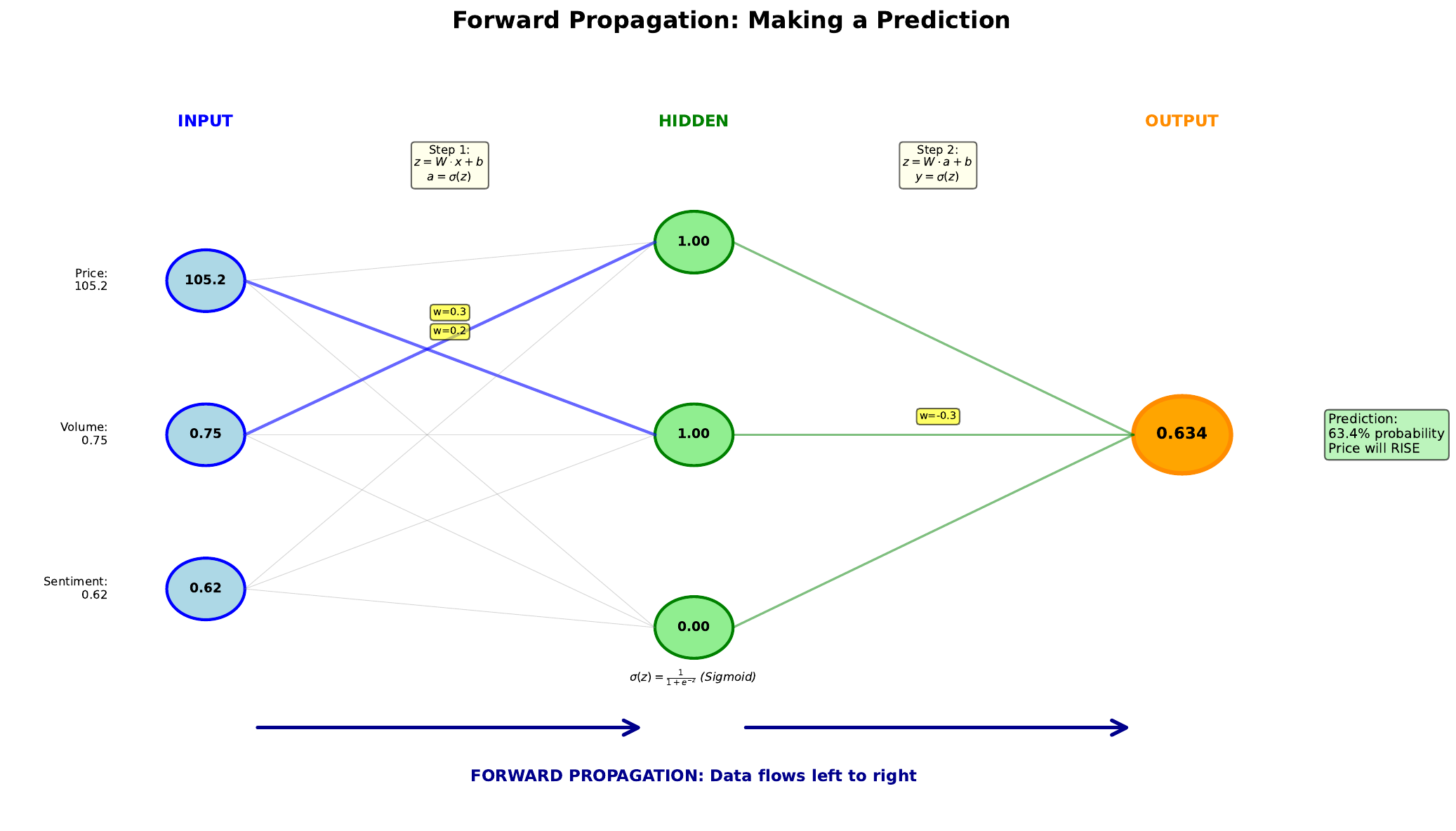
Forward propagation is the process of computing a network’s output given an input. Data flows forward from input layer through hidden layers to the output layer - hence the name.
At each layer, we perform two operations:
- Linear transformation: Multiply inputs by weights and add bias (z = Wx + b)
- Non-linear activation: Apply activation function (a = f(z))
The output of one layer becomes the input to the next. When data reaches the output layer, we have our prediction. During training, we compare this prediction to the true value to calculate error.
For a trading application, forward propagation answers: “Given today’s market data, what does the network predict about tomorrow’s price?”
Visual
Key Formulas
Hidden layer computation: \(z^{[1]} = W^{[1]} x + b^{[1]}\) \(a^{[1]} = \sigma(z^{[1]})\)
Output layer computation: \(z^{[2]} = W^{[2]} a^{[1]} + b^{[2]}\) \(\hat{y} = \sigma(z^{[2]})\)
Where:
- x = input features
- W^[l] = weight matrix for layer l
- b^[l] = bias vector for layer l
- z^[l] = pre-activation values
- a^[l] = activation values (layer output)
- y-hat = predicted output
Intuitive Explanation
Imagine a relay race where each runner transforms the baton before passing it:
- Start: Raw market data (price = 105.2, volume = 0.75, sentiment = 0.62)
- Hidden layer: Each neuron “weighs” this data, adds its perspective, and outputs a transformed signal
- Output layer: The final neuron combines all hidden signals into a single prediction
- Finish: Probability of price increase (e.g., 74.2%)
The weights determine how much each neuron “listens” to each input. Training adjusts these weights to improve predictions.
Practice Problems
Problem 1
A network has 2 inputs, 2 hidden neurons, and 1 output. Given:
- Input: x = [1.0, 0.5]
- Hidden weights: W1 = [[0.2, 0.4], [0.6, 0.3]]
- Hidden bias: b1 = [0.1, -0.1]
Calculate z1 (pre-activation for hidden layer).
Solution
For hidden neuron 1: $$z_1^{[1]} = 0.2(1.0) + 0.4(0.5) + 0.1 = 0.2 + 0.2 + 0.1 = 0.5$$ For hidden neuron 2: $$z_2^{[1]} = 0.6(1.0) + 0.3(0.5) + (-0.1) = 0.6 + 0.15 - 0.1 = 0.65$$ **z1 = [0.5, 0.65]**Problem 2
Continuing from Problem 1, apply sigmoid activation to get a1 (hidden layer output).
Solution
$$a_1^{[1]} = \sigma(0.5) = \frac{1}{1+e^{-0.5}} = \frac{1}{1+0.607} = 0.622$$ $$a_2^{[1]} = \sigma(0.65) = \frac{1}{1+e^{-0.65}} = \frac{1}{1+0.522} = 0.657$$ **a1 = [0.622, 0.657]**Problem 3
Complete the forward pass. Given output weights W2 = [0.5, 0.7] and bias b2 = -0.3, calculate the final prediction.
Solution
$$z^{[2]} = 0.5(0.622) + 0.7(0.657) + (-0.3)$$ $$z^{[2]} = 0.311 + 0.460 - 0.3 = 0.471$$ $$\hat{y} = \sigma(0.471) = \frac{1}{1+e^{-0.471}} = \frac{1}{1+0.624} = 0.616$$ **Final prediction: 61.6% probability** The network predicts "BUY" (probability > 50%).Key Takeaways
- Forward propagation computes output from input layer to output layer
- Each layer: linear transformation (Wx + b) then activation (f)
- All neurons in a layer compute in parallel
- The final output is the network’s prediction
- No learning happens during forward propagation - just computation
(c) Joerg Osterrieder 2025