Exercises
This page collects all practice problems from the course in one place for self-study and review.
Part 1: Foundations (Topics 01-04)
Topic 01: Biological Neuron
Problem 1.1: A neuron receives three inputs: x1 = 0.5, x2 = 0.8, x3 = 0.2. The weights are w1 = 0.4, w2 = 0.3, w3 = 0.5, and the bias is b = -0.1. Calculate the weighted sum z.
Solution
z = (0.4)(0.5) + (0.3)(0.8) + (0.5)(0.2) + (-0.1) = 0.20 + 0.24 + 0.10 - 0.10 = 0.44Problem 1.2: In the biological neuron, what structure is analogous to the weights in an artificial neuron?
Solution
The synaptic strengths are analogous to weights. Both determine how much each input contributes to the final decision, and both change with learning.Topic 02: Single Neuron Computation
Problem 2.1: Given inputs Price = 1.2, Volume = 0.8, Sentiment = 0.6, with weights w1 = 0.5, w2 = 0.3, w3 = 0.4 and bias b = -0.5, calculate the weighted sum z.
Solution
z = (0.5)(1.2) + (0.3)(0.8) + (0.4)(0.6) + (-0.5) = 0.60 + 0.24 + 0.24 - 0.50 = 0.58Problem 2.2: Using z = 0.58, calculate the sigmoid output. What is the predicted probability?
Solution
y = 1/(1 + e^-0.58) = 1/(1 + 0.560) = 0.641 = 64.1% probability of price increase (BUY signal)Part 2: Building Blocks (Topics 05-08)
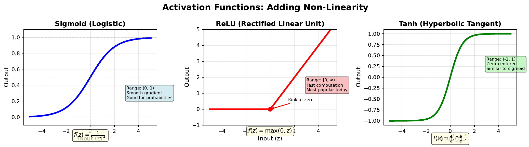
Topic 05: Activation Functions
Problem 3.1: Calculate the output of sigmoid, ReLU, and tanh for z = 2.0.
Solution
- Sigmoid: 1/(1+e^-2) = 0.881 - ReLU: max(0, 2.0) = 2.0 - Tanh: (e^2 - e^-2)/(e^2 + e^-2) = 0.964Problem 3.2: Calculate the output of each function for z = -1.5.
Solution
- Sigmoid: 1/(1+e^1.5) = 0.182 - ReLU: max(0, -1.5) = 0 - Tanh: (e^-1.5 - e^1.5)/(e^-1.5 + e^1.5) = -0.905Topic 06: Linear Limitation
Problem 4.1: Consider the AND function. Is it linearly separable? Find weights and bias that work.
Solution
Yes, AND is linearly separable. Solution: w1 = 1, w2 = 1, b = -1.5 - (0,0): 0 + 0 - 1.5 = -1.5 < 0 -> 0 - (0,1): 0 + 1 - 1.5 = -0.5 < 0 -> 0 - (1,0): 1 + 0 - 1.5 = -0.5 < 0 -> 0 - (1,1): 1 + 1 - 1.5 = 0.5 > 0 -> 1Problem 4.2: Explain why XOR cannot be solved with a single neuron.
Solution
XOR requires (0,0)->0, (0,1)->1, (1,0)->1, (1,1)->0. The Class 1 points (0,1) and (1,0) are diagonally opposite from Class 0 points (0,0) and (1,1). No single straight line can separate diagonal corners - the classes are interleaved.Part 3: Architecture (Topics 09-12)
Topic 09: Network Architecture
Problem 5.1: A network has architecture [10, 8, 6, 1]. How many total parameters?
Solution
- Layer 1: 10*8 + 8 = 88 - Layer 2: 8*6 + 6 = 54 - Layer 3: 6*1 + 1 = 7 - Total: 149 parametersProblem 5.2: You have 1,000 training samples. Is architecture [50, 100, 100, 50, 1] appropriate?
Solution
No. Parameters = 5,100 + 10,100 + 5,050 + 51 = 20,301. With 20x more parameters than samples, severe overfitting is likely. Use a smaller network like [50, 20, 1] with ~1,041 parameters.Topic 10: Forward Propagation
Problem 6.1: Network with 2 inputs, 2 hidden neurons. Input x = [1.0, 0.5], weights W1 = [[0.2, 0.4], [0.6, 0.3]], bias b1 = [0.1, -0.1]. Calculate z1.
Solution
z1 = [0.2(1.0) + 0.4(0.5) + 0.1, 0.6(1.0) + 0.3(0.5) + (-0.1)] = [0.5, 0.65]Problem 6.2: Apply sigmoid to z1 = [0.5, 0.65] to get a1.
Solution
a1 = [sigmoid(0.5), sigmoid(0.65)] = [0.622, 0.657]Part 4: Learning Process (Topics 13-16)
Topic 13: Loss Landscape
Problem 7.1: Calculate cross-entropy loss for y = 1, y-hat = 0.9.
Solution
L = -[1*log(0.9) + 0*log(0.1)] = -log(0.9) = 0.105Problem 7.2: Calculate loss for y = 1, y-hat = 0.1 (bad prediction).
Solution
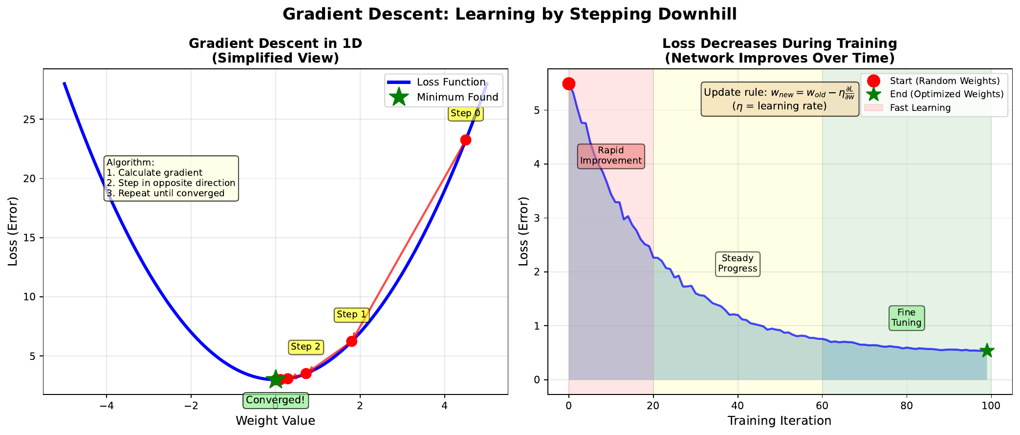
L = -log(0.1) = 2.303 (22x worse than good prediction)Topic 14: Gradient Descent
Problem 8.1: Current weight w = 2.5, learning rate = 0.1, gradient = 0.8. Calculate new weight.
Solution
w_new = 2.5 - 0.1 * 0.8 = 2.5 - 0.08 = 2.42Problem 8.2: After training, gradient becomes 0.001. What does this indicate?
Solution
Near convergence - we're close to a minimum. Weight updates are tiny (0.1 * 0.001 = 0.0001), training is essentially complete.Part 5: Application (Topics 17-20)
Topic 17: Market Prediction Data
Problem 9.1: Price min=95, max=105, current=102. Calculate min-max normalized value.
Solution
x_norm = (102 - 95)/(105 - 95) = 7/10 = 0.70Problem 9.2: Volume mean=1M, std=250K, today=1.5M. Calculate z-score.
Solution
z = (1,500,000 - 1,000,000)/250,000 = 2.0 standard deviations above averageTopic 18: Prediction Results
Problem 10.1: Network makes 140 correct predictions out of 200. Calculate accuracy and improvement over random baseline.
Solution
Accuracy = 140/200 = 70%. Improvement = 70% - 50% = 20 percentage pointsTopic 15: Overfitting vs Underfitting
Problem 17.1: Training loss = 0.15, validation loss = 0.65. Diagnosis?
Solution
Overfitting. Low training loss but high validation loss indicates memorization. Solutions: more data, regularization, simpler model, early stopping.Problem 17.2: Training loss = 0.55, validation loss = 0.58. Diagnosis?
Solution
Underfitting. Both losses are high with small gap. Solutions: more complex model, train longer, better features, reduce regularization.Topic 19: Confusion Matrix (NEW)
Problem 19.1: TP=40, FP=15, TN=35, FN=10. Calculate precision, recall, F1.
Solution
- Precision = 40/(40+15) = 72.7% - Recall = 40/(40+10) = 80.0% - F1 = 2*(0.727*0.800)/(0.727+0.800) = 76.2%Topic 20: Trading Backtest (NEW)
Problem 20.1: Transaction cost is 0.1% per trade. Strategy trades 200 times per year. Total cost impact?
Solution
Total cost = 200 * 0.1% = 20 percentage points of returns lost to trading costs. High-frequency strategies need very high accuracy or low costs.Challenge Problems
Challenge 1: Complete Forward Pass
A network has architecture [2, 3, 1] with:
- W1 = [[0.1, 0.2], [0.3, 0.4], [0.5, 0.6]]
- b1 = [0.1, 0.2, 0.3]
- W2 = [0.5, 0.3, 0.2]
- b2 = [-0.5]
- Input: x = [1.0, 2.0]
Calculate the final output using sigmoid activation.
Solution
Hidden layer: - z1[0] = 0.1*1.0 + 0.2*2.0 + 0.1 = 0.6 -> a1[0] = sigmoid(0.6) = 0.646 - z1[1] = 0.3*1.0 + 0.4*2.0 + 0.2 = 1.3 -> a1[1] = sigmoid(1.3) = 0.786 - z1[2] = 0.5*1.0 + 0.6*2.0 + 0.3 = 2.0 -> a1[2] = sigmoid(2.0) = 0.881 Output layer: - z2 = 0.5*0.646 + 0.3*0.786 + 0.2*0.881 - 0.5 = 0.323 + 0.236 + 0.176 - 0.5 = 0.235 - y = sigmoid(0.235) = 0.558 Final output: 55.8% probability (BUY)Challenge 2: Gradient Descent Simulation
Starting weight w = 5.0. Loss function L(w) = (w - 2)^2. Learning rate = 0.1.
Perform 5 gradient descent steps and track the weight values.
Solution
dL/dw = 2(w - 2) Step 1: w = 5.0, grad = 2(5-2) = 6, w_new = 5.0 - 0.1*6 = 4.4 Step 2: w = 4.4, grad = 2(4.4-2) = 4.8, w_new = 4.4 - 0.1*4.8 = 3.92 Step 3: w = 3.92, grad = 2(3.92-2) = 3.84, w_new = 3.92 - 0.1*3.84 = 3.536 Step 4: w = 3.536, grad = 2(3.536-2) = 3.07, w_new = 3.536 - 0.1*3.07 = 3.229 Step 5: w = 3.229, grad = 2(3.229-2) = 2.46, w_new = 3.229 - 0.1*2.46 = 2.983 Weight sequence: 5.0 -> 4.4 -> 3.92 -> 3.536 -> 3.229 -> 2.983 Converging toward minimum at w = 2.(c) Joerg Osterrieder 2025