A6: How AMMs Set Prices — The Constant Product Formula
Introduction
An AMM (Automated Market Maker) is a piece of software that lets people trade one cryptocurrency for another without needing a human broker or traditional exchange. AMMs use the constant product formula x * y = k where:
- x and y are the quantities of two tokens in a liquidity pool (a shared pot of funds that anyone can trade against)
- k is a constant that never changes
When you buy token A, you add token B to the pool and remove token A. This changes the ratio y/x, which automatically changes the price. Slippage (the difference between the expected price and the actual price you pay) increases with trade size because larger trades move the ratio more.
Your Task
You will explore how different pool parameters affect slippage by modifying the baseline constant product AMM model. Create a 7-slide Marp presentation analyzing three variations and one open extension.
Baseline Model
- Pool depth: k = 1,000,000
- Initial reserves: x₀ = 1000, y₀ = 1000 (balanced pool, price = 1.0)
- Spot price formula: P = y/x
- Trade formula: When you buy Δx of token X, you pay Δy = k/(x − Δx) − y tokens of Y
Variations to Analyze
Variation 1: Increase pool depth
- Set k = 10,000,000 (10x larger pool, meaning √(10M) ≈ 3162 of each token initially)
- How does slippage for a 100-token trade change compared to baseline?
- Why does deeper liquidity improve prices?
Variation 2: Imbalanced pool
- Set initial reserves: x₀ = 500, y₀ = 2000 (initial price = y/x = 4.0 instead of 1.0)
- Keep k = 1,000,000 (so x₀ * y₀ = k still holds)
- How does the curve shape differ?
- What happens to slippage when buying X vs buying Y?
Variation 3: Add 0.3% swap fee
- Apply fee to output: effective output = amount_out * 0.997
- Compute effective slippage for trades of [10, 50, 100, 200, 500] tokens
- Compare to baseline (no fee)
- How much does the fee add to total slippage?
Open Extension: Pool Depth Comparison
- Create a chart comparing slippage between k = 1M and k = 10M on the same axes
- Show slippage curves for trade sizes from 10 to 500 tokens
- What is the percentage reduction in slippage at different trade sizes?
Deliverables
- 7-slide Marp presentation (
model-answer-presentation.md):- Slide 1: Title + citation (Adams et al. 2021 — Uniswap v3 Core)
- Slide 2: The Model — formula explanation
- Slide 3: Baseline results with baseline chart
- Slide 4: Variation 1 results with variation chart
- Slide 5: Variation 2 results
- Slide 6: Variation 3 results with fee comparison
- Slide 7: Key insights — why pool depth matters
- Python chart (
chart_varied.py):- 2×2 subplot grid (16×12 inches)
- Panel 1: Baseline — constant product curve with trade arrows for 100 and 500 token trades
- Panel 2: Variation 1 — k = 10M, same trades, show reduced slippage
- Panel 3: Variation 2 — x₀ = 500, y₀ = 2000, show asymmetric curve
- Panel 4: Variation 3 — bar chart comparing slippage with and without 0.3% fee for trade sizes [10, 50, 100, 200, 500]
- Use
np.random.seed(42)for reproducibility - Save to
chart_varied.pdfandchart_varied.png
How to Run
Use Google Colab (free, no installation required):
- Go to colab.research.google.com
- Upload
chart_varied.py - Run the script (Runtime → Run all)
- Download generated PNG/PDF from the Files panel (left sidebar)
For the Marp presentation:
- Install the Marp extension in VS Code, or
- Use the online Marp editor at marp.app
Time Allocation
- Analysis and coding: 45 minutes
- Presentation preparation: 10 minutes
- Total: 55 minutes
Learning Objectives
By completing this assignment, you will:
- Understand how the constant product formula x * y = k automatically sets prices
- See why larger trades suffer worse slippage (convex, not linear)
- Appreciate why liquidity mining exists (deep pools = better prices)
- Recognize the importance of pool balance and fee structure
- Practice presenting quantitative financial analysis visually
Grading Rubric (100 points)
| Component | Points | Criteria |
|---|---|---|
| Variation 1 analysis | 20 | Correct k = 10M calculation, slippage comparison |
| Variation 2 analysis | 20 | Correct imbalanced pool, asymmetric curve explanation |
| Variation 3 analysis | 20 | Fee calculation correct, slippage comparison table |
| Chart quality | 20 | All 4 panels correct, annotations clear, professional |
| Presentation clarity | 15 | Logic flow, key insights highlighted, visuals support text |
| Open extension | 5 | Thoughtful comparison, actionable insight |
References
Adams, H., Zinsmeister, N., Salem, M., Keefer, R., & Robinson, D. (2021). Uniswap v3 Core. Retrieved from https://uniswap.org/whitepaper-v3.pdf
Show Model Answer Presentation (7 slides)
Slide 3 — Baseline Results
Baseline Results (k = 1M, x₀ = y₀ = 1000)
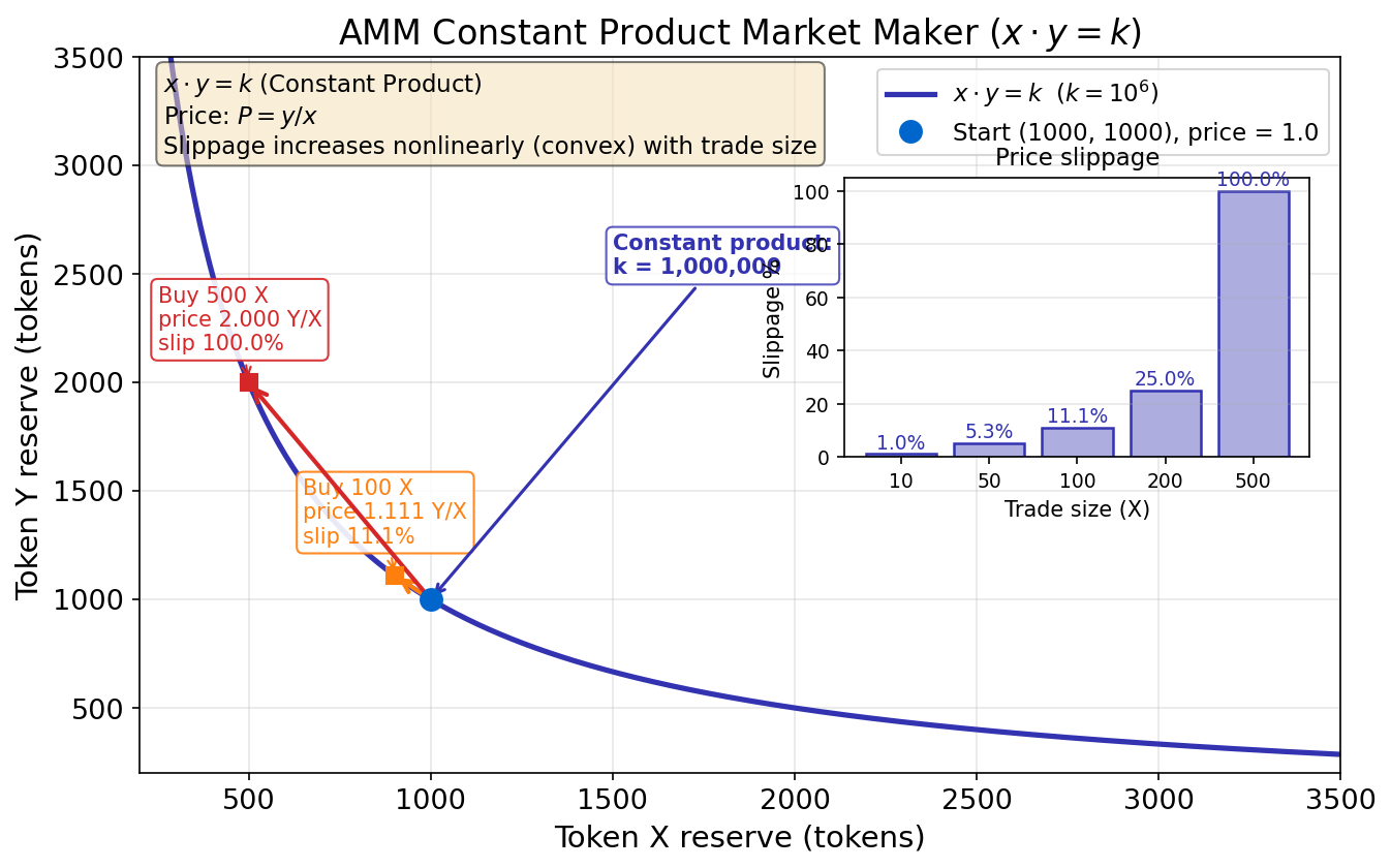
Observations:
- Trade 100 X: Costs 111 Y → effective price 1.111 Y/X → 11.1% slippage
- Trade 500 X: Costs 1000 Y → effective price 2.0 Y/X → 100% slippage
- Slippage grows nonlinearly (convex function)
Slide 4 — Variation 1
Variation 1: Deeper Pool (k = 10M)
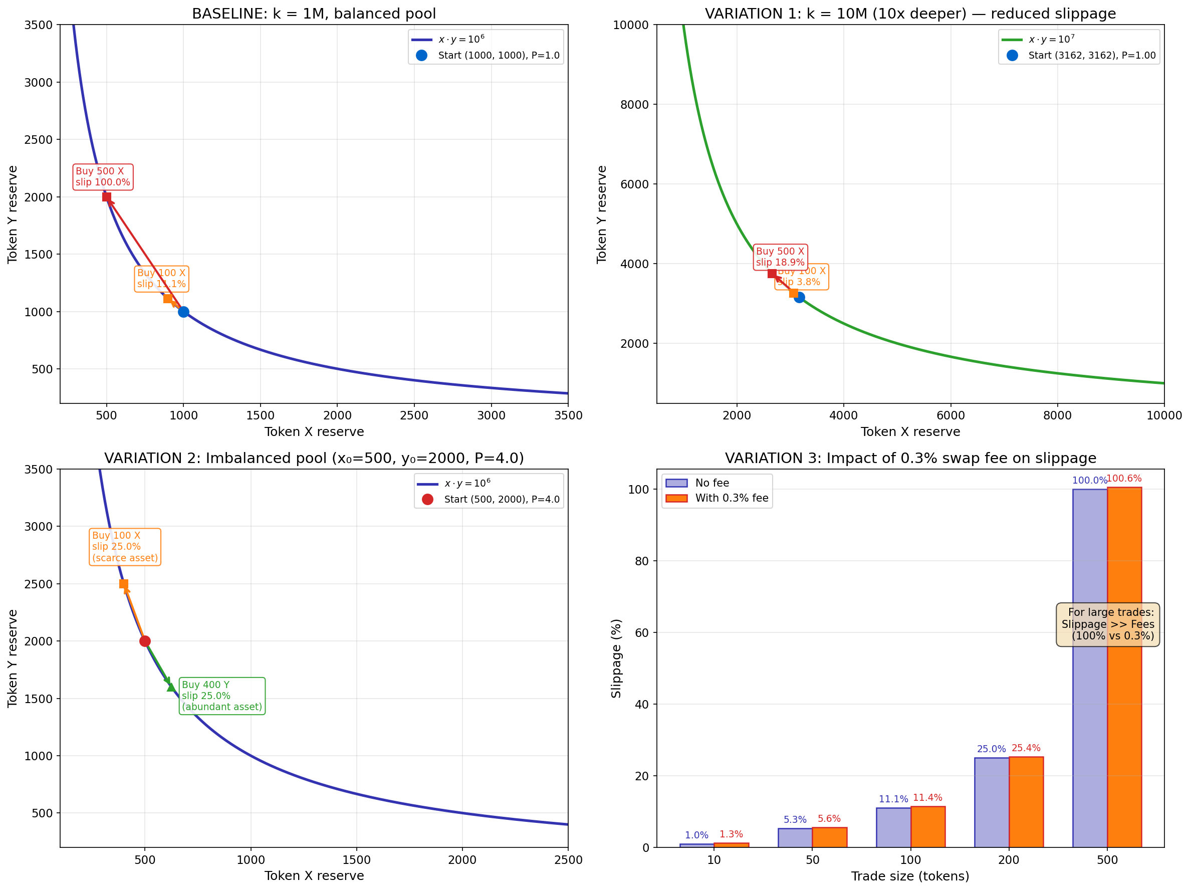
(Panel 2: k = 10M — note reduced slippage)
Results:
- Same 100 X trade now costs ~103.8 Y → ~3.8% slippage (down from 11.1%)
- Slippage reduction: ~66% improvement with 10x deeper liquidity
- Why?: Larger k means flatter curve → smaller percentage change in y/x ratio
Key Insight: This is why liquidity mining exists — deeper pools attract traders with better prices.
Slide 5 — Variation 2
Variation 2: Imbalanced Pool (x₀ = 500, y₀ = 2000)
(Panel 3: Asymmetric curve with initial price P = 4.0)
Results:
- Initial price P = y/x = 2000/500 = 4.0 Y/X (not 1.0)
- Curve is steeper on the X-side (buying X is expensive)
- Curve is flatter on the Y-side (buying Y is cheaper)
- Asymmetry: Traders pay more slippage when buying the scarce asset (X)
Implication: Arbitrageurs will rebalance the pool toward x₀ = y₀ if external price differs.
Slide 6 — Variation 3
Variation 3: Adding 0.3% Swap Fee
(Panel 4: Slippage comparison with and without fee)
Fee Model: Effective output = amount_out × 0.997
| Trade Size (X) | Slippage (no fee) | Slippage (with 0.3% fee) | Fee Impact |
|---|---|---|---|
| 10 | 1.0% | 1.3% | +0.3 pp |
| 50 | 5.3% | 5.6% | +0.3 pp |
| 100 | 11.1% | 11.4% | +0.3 pp |
| 200 | 25.0% | 25.4% | +0.4 pp |
| 500 | 100.0% | 100.6% | +0.6 pp |
Observation: Fee adds constant ~0.3 percentage points. For large trades, slippage dominates fees.