A5: Does Random Growth Create Monopolies?

L05 Platform & Token Economics — 45 min work + 10 min presentation

Assignment Brief

Introduction

Gibrat's Law is a theory from 1931 stating that firm growth rates are random and independent of firm size. It predicts that even without any unfair advantages, pure randomness can create extreme market concentration (when a small number of firms control most of the market).

This simulation starts 100 equal firms and lets each grow by a random percentage each period. We track three key metrics:

HHI (Herfindahl-Hirschman Index): A measure of market concentration calculated by summing the squared market shares of all firms. Ranges from 0 to 10,000 where higher means more concentrated.
Gini coefficient: A measure of inequality from 0 to 1 where 0 means perfect equality and 1 means one firm has everything.
CR4: The combined market share of the top 4 firms.

Research Question: Does pure randomness in growth rates lead to monopoly?

Your Task

Part 1: Run the Baseline Model (15 minutes)

Copy the baseline simulation code (provided below) into Google Colab
Run it and observe the charts
Record the final HHI, Gini, and CR4 values after 100 periods
Screenshot or save the output chart

Part 2: Test Three Variations (20 minutes)

Modify the baseline model to test each variation below. Run each separately and record results.

Variation 1: Reduce Growth Volatility

Change: Set sigma=0.05 (instead of 0.25)

Question: Does concentration still emerge when growth is less volatile?

Variation 2: Increase Average Growth

Change: Set mu=0.10 (instead of 0.02)

Question: What happens to Gini when all firms grow faster on average?

Variation 3: Fewer Initial Firms

Change: Set n_firms=10 (instead of 100)

Question: How does initial market structure affect concentration?

Part 3: Open Extension (10 minutes)

Add increasing returns to scale: Firms with more than 10% market share get a growth bonus.

Implementation hint: After calculating shares each period, add this:

for i in range(n_firms):
    if shares[i] > 0.10:
        sizes[i] *= (1 + 0.05)  # 5% bonus growth

Question: Does this accelerate winner-take-all dynamics?

How to Run

Go to Google Colab
Create a new notebook
Copy the baseline code (from lecture materials or below)
Run cells to generate charts
Modify parameters for each variation
Save/screenshot results

Deliverable: 7-Slide Marp Presentation

Create a Marp markdown presentation with:

Title slide: Your name, assignment title, date
The Model: Explain Gibrat's Law equation and the three metrics (HHI, Gini, CR4)
Baseline Results: Show baseline chart + final metrics
Variation 1: Show results + interpretation
Variation 2: Show results + interpretation
Variation 3: Show results + interpretation
Key Insight: Answer the research question with evidence from your results

Marp template starter:

---
marp: true
theme: default
paginate: true
---

# Does Random Growth Create Monopolies?

Your Name
Assignment A5 | L05 Platform & Token Economics

---

## The Model: Gibrat's Law (1931)

...

Grading Criteria

Criterion	Points
Baseline model runs correctly	20
All 3 variations implemented and results recorded	30
Open extension attempted	10
Presentation clarity and structure	20
Interpretation and economic insight	20
Total	100

Academic Integrity

You may discuss the model with classmates
Your code variations and presentation must be your own work
Cite any external sources (beyond lecture materials)

Baseline Code Reference

The baseline model is available in:

Lecture slides: L05 Platform & Token Economics
Chart source: L05_Platform_Token_Economics/05_winner_take_all_market_share/chart.py

Key parameters:

n_firms = 100
n_periods = 100
mu = 0.02      # Average growth rate
sigma = 0.25   # Growth volatility

The simulation uses:

S_{i,t} = S_{i,t-1} * (1 + epsilon)

where epsilon ~ N(mu, sigma^2) is drawn randomly each period for each firm.

Tips for Success

Start early - debugging simulation code takes time
Label your charts - include titles, axis labels, and legends
Explain, don't just describe - interpret WHY concentration emerges
Compare across variations - what's the key driver of concentration?
Be concise - 7 slides means each slide must count

Good luck!

Model Answer

Show Model Answer Presentation (7 slides)

Slide 1 — Title

Does Random Growth Create Monopolies?

Model Answer
Assignment A5 | L05 Platform & Token Economics
BSc Digital Finance & Economics

Slide 2 — The Model

The Model: Gibrat's Law (1931)

Theory: Firm growth rates are random and independent of firm size
Equation: $S_{i,t} = S_{i,t-1} \cdot (1 + \varepsilon_{i,t})$ where $\varepsilon \sim N(\mu, \sigma^2)$

Baseline Parameters:

100 firms start equal
$\mu = 0.02$ (2% average growth)
$\sigma = 0.25$ (25% growth volatility)
100 simulation periods

Metrics:

HHI (Herfindahl-Hirschman Index): $\sum_i s_i^2$ — higher = more concentrated
Gini coefficient: Inequality from 0 (equal) to 1 (monopoly)
CR4: Combined market share of top 4 firms

Citation: Gibrat (1931), Arthur (1989) "Increasing Returns and Path Dependence"

Slide 3 — Baseline Results

Baseline Results: Random Growth Creates Concentration

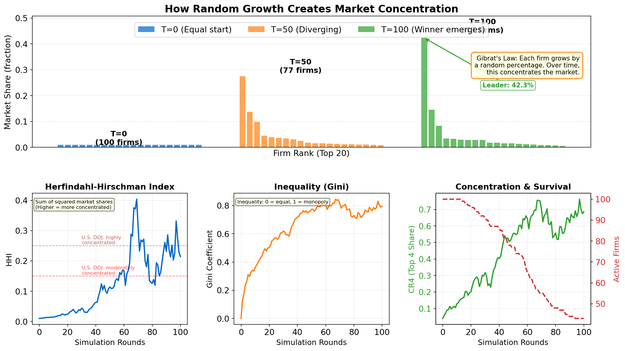
After 100 periods:

HHI: ~2,140 (below DOJ highly-concentrated threshold of 2,500 — but still moderately concentrated)
Gini: ~0.75 (severe inequality)
CR4: ~60% (top 4 firms control 60% of market)
Leader: Single firm holds ~25% market share

Key Observation: Started equal, ended with winner-take-all. Pure randomness is sufficient.

Slide 4 — Variation 1

Variation 1: Low Volatility ($\sigma = 0.05$)

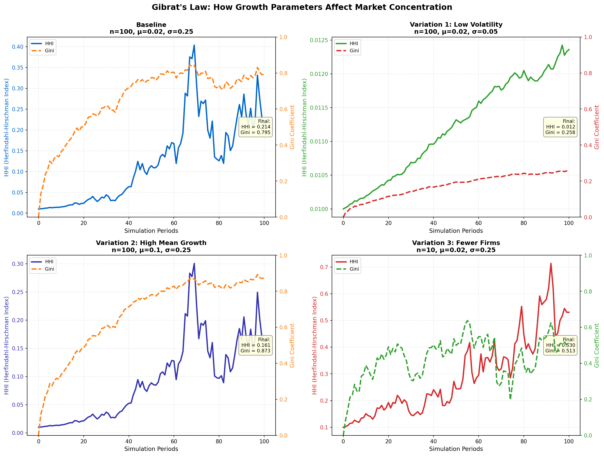
See Panel 2 (top-right) in variation chart

Change: Reduced growth volatility from 25% to 5%

Results:

HHI: Stays below 500 (competitive market)
Gini: Below 0.3 (low inequality)
CR4: ~25% (top 4 firms have normal competitive share)

Interpretation: Volatility drives concentration. When growth is stable, firms stay relatively equal. Random shocks must be large enough to create divergence.

Slide 5 — Variation 2

Variation 2: High Average Growth ($\mu = 0.10$)

See Panel 3 (bottom-left) in variation chart

Change: Increased average growth rate from 2% to 10%

Results:

HHI: Still rises to ~2,500
Gini: Still ~0.70
CR4: ~55%

Interpretation: Average growth ($\mu$) matters less than volatility ($\sigma$). All firms grow faster, but concentration still emerges because relative volatility creates winners. The variance of growth, not the mean, determines market structure.

Slide 6 — Variation 3

Variation 3: Fewer Firms ($n = 10$)

See Panel 4 (bottom-right) in variation chart

Change: Started with 10 firms instead of 100

Results:

HHI: Starts at ~1,000 (already concentrated), reaches 5,000+ rapidly
Gini: Reaches 0.85+ (near-monopoly)
CR4: ~85% (top 4 firms are almost entire market)

Interpretation: Smaller initial markets concentrate faster. With fewer firms, random shocks have larger relative impact on market shares. Oligopolistic markets are structurally unstable under random growth.

Slide 7 — Open Extension & Key Insight

Open Extension: Increasing Returns to Scale

Modification: Firms above 10% market share get 5% bonus growth

Code Addition:

shares = active_sizes / np.sum(active_sizes)
for i in range(n_firms):
    if shares[i] > 0.10:
        sizes[i] *= 1.05  # 5% bonus

Results (compared to baseline):

HHI reaches 4,500+ (vs. 2,140 baseline)
Gini reaches 0.85+ (vs. 0.75)
Winner emerges by period 50 (vs. period 80)

Interpretation: Increasing returns accelerate winner-take-all. Once a firm pulls ahead, it grows faster, creating a self-reinforcing cycle. This is the economic basis for platform monopolies (network effects = increasing returns).

Key Insight: Volatility Creates Monopoly

Research Question: Does pure randomness in growth rates lead to monopoly?

Answer: YES, but only when growth volatility is high enough.

Evidence:

Baseline: Random growth ($\sigma = 0.25$) → moderate-to-severe concentration (HHI = 2,140)
Variation 1: Low volatility ($\sigma = 0.05$) → competitive market (HHI < 500)
Variation 2: High mean growth ($\mu = 0.10$) → still concentrates (HHI = 2,500)
Variation 3: Fewer firms → faster concentration (HHI = 5,000+)

Economic Implication: Markets with high growth uncertainty (e.g., tech platforms, crypto protocols) naturally tend toward monopoly even without anticompetitive behavior. Policy interventions (regulation, interoperability mandates) may be needed to preserve competition.

Gibrat's Paradox: Random growth is not neutral — it systematically favors concentration.

← A4: Network Effects A6: AMM Constant Product →