A8: How Financial Crises Spread Through Networks
Assignment Brief
Introduction
When one bank fails, its losses can spread to connected banks, triggering a cascade (a chain reaction where failures cause more failures). This model simulates financial contagion (the spread of financial distress from one institution to others through direct connections) on a random network of 20 financial institutions.
Each institution has a capital buffer $B_i$ (money set aside to absorb losses -- like a safety cushion). When institution $i$ fails, it spreads losses to its neighbors. If a neighbor's accumulated losses exceed its buffer, it also fails -- creating a cascade.
The formula for losses received by institution $i$ is:
$$\text{Loss}_i = \sum_{j \in \text{failed neighbors}} \frac{\text{Loss}_j}{\text{degree}_j}$$where $\text{degree}_j$ is the number of connections that institution $j$ has.
Your Task
Run the baseline simulation, then implement three variations to explore how different factors affect systemic risk. Create a 7-slide presentation (using Marp or PowerPoint) summarizing your findings.
Variations to Implement
Variation 1: Double All Buffers
Change: On line 42, modify the capital buffer range from [0.05, 0.20] to [0.10, 0.40]:
buffers = np.random.uniform(0.10, 0.40, N)Question: How many nodes fail now compared to baseline? What does this tell you about capital requirements as a policy tool?
Variation 2: Increase Network Density
Change: On line 36, make the network more connected by changing < 0.3 to < 0.7:
adj = np.random.rand(N, N) < 0.7Question: Does more connectivity help or hurt financial stability? Why might dense networks be "robust-yet-fragile"?
Variation 3: Multiple Initial Failures
Change: After line 53, add two more initial failures:
failed[shock_node] = True
failed[1] = True
failed[2] = True
Also update line 56 to reflect 3 initial failures:
round_failures = [3] # Initial shocksQuestion: How does the cascade differ when 3 banks fail simultaneously versus a single shock?
Open Extension (Optional)
Add a circuit breaker mechanism: any node that has lost 50% of its buffer freezes all outgoing connections (stops spreading losses to neighbors). This simulates emergency liquidity injections or regulatory interventions.
Implementation hint: Track a new boolean array frozen and modify the loss propagation loop to skip frozen nodes.
How to Run
- Upload the provided
chart.pyfile to Google Colab - Run the baseline version first to understand the output
- Make each variation change one at a time
- Save the network visualizations and failure counts for each variation
- Create your presentation comparing all four scenarios
Deliverables
Submit a 7-slide presentation (PDF or PPTX):
- Title slide with your name and the reference: Acemoglu et al. (2015) - Systemic Risk and Network Topology
- The Model -- explain the mechanics (20 nodes, random connections, capital buffers, loss propagation formula)
- Baseline Results -- network visualization + total failures
- Variation 1 -- doubled buffers analysis
- Variation 2 -- dense network analysis
- Variation 3 -- multiple shocks analysis
- Key Insights -- what did you learn about systemic risk and network structure?
Time Allocation
- 45 minutes: Run simulations and analyze results
- 10 minutes: Create presentation slides
Assessment Criteria
- Correctness: All three variations implemented correctly (30%)
- Analysis: Clear explanations of how each change affects contagion (40%)
- Insight: Understanding of the "robust-yet-fragile" paradox and policy implications (20%)
- Presentation: Clear visuals and concise explanations (10%)
Learning Objectives
By completing this assignment, you will:
- Understand how financial contagion spreads through networks
- Recognize the counterintuitive effects of network density on systemic risk
- Evaluate the effectiveness of capital buffers as a policy tool
- Appreciate why regulators monitor interconnectedness in financial systems
Model Answer
Show Model Answer Presentation
Slide 3 of 7
Baseline Results: Single Shock Cascade
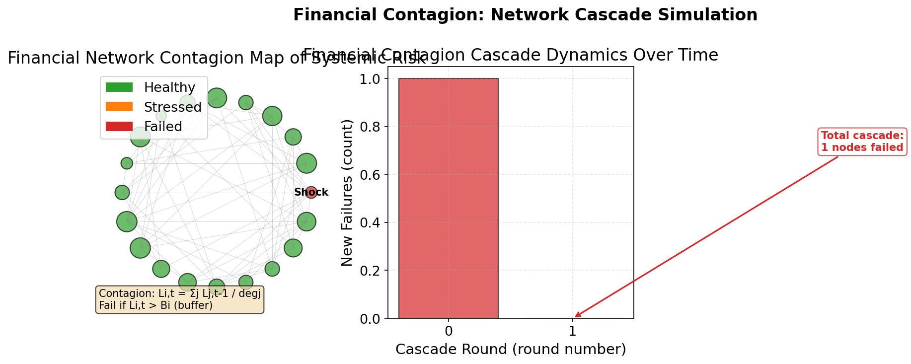
Observations:
- Initial shock to node 0 (marked "Shock")
- Cascade spreads through network connections
- Multiple rounds of failures (shown in bar chart)
- Some nodes become stressed (orange) but don't fail
- Total failures depend on network structure and buffer distribution
Slide 4 of 7
Variation 1: Doubled Capital Buffers
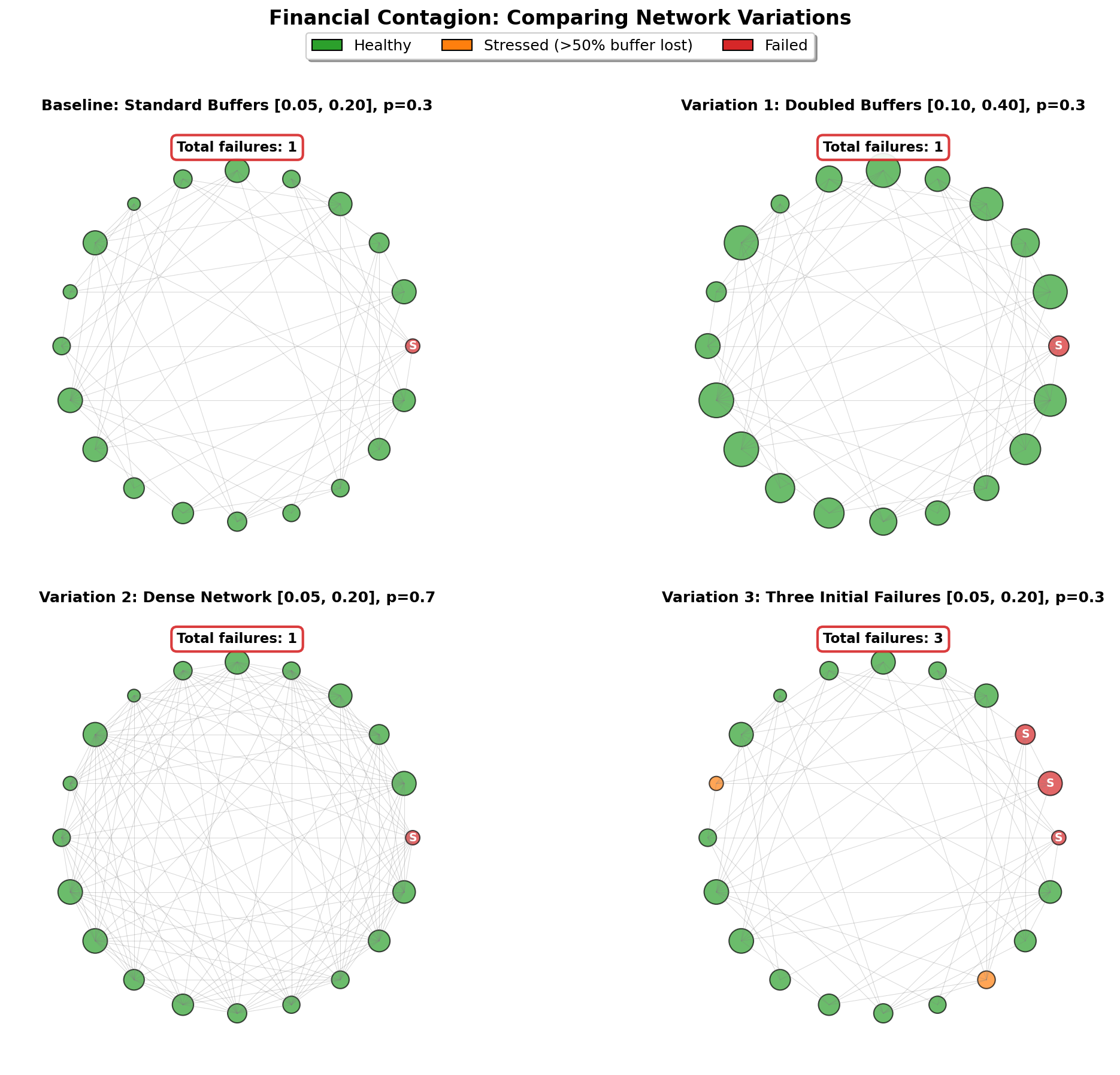
Change: Buffers increased from [0.05, 0.20] to [0.10, 0.40]
Result: Significantly fewer failures
Policy Implication:
Capital requirements are the most effective defense against systemic risk. Even modest increases in buffers can prevent cascades.
Trade-off: Higher capital requirements reduce bank profitability and may restrict lending.