Pre-Class Discovery: Logistic Regression

Activity 1

"Approve or Deny?"

Income ($k)	Debt Ratio	Credit Score	Outcome
35	0.65	580	Denied
85	0.20	750	Approved
42	0.55	620	Denied
120	0.15	800	Approved
55	0.45	660	Denied
95	0.30	720	Approved
38	0.70	590	Denied
110	0.25	780	Approved

Your Task

Sort by income -- does higher income always mean approval?
Which single feature best separates approved from denied?
Can you write a simple rule (e.g., "approve if credit score > __")?

Reveal Solution

No single feature perfectly separates the outcomes. We need a model that combines features and outputs a probability, not just yes/no. Logistic regression does exactly this: it maps a weighted sum of features through the sigmoid function to produce a probability between 0 and 1.

Activity 2

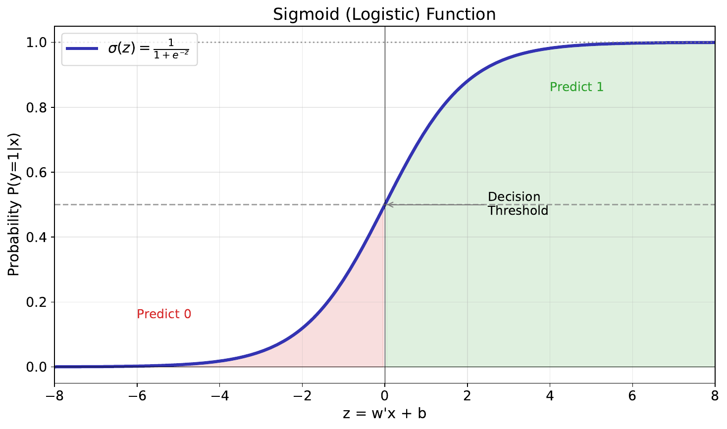
"The S-Shaped Curve"

Sigmoid function mapping any real number to a probability between 0 and 1

Your Task

What happens at the extremes -- very large or very small input?
What is the output when the input equals 0?
Why is this S-shape useful for modeling probabilities?

Reveal Solution

The sigmoid function $\sigma(z) = \frac{1}{1 + e^{-z}}$ maps any number to (0, 1). At extremes, it saturates near 0 or 1 (high confidence). At $z=0$, the output is 0.5 (maximum uncertainty). It's perfect for probabilities because it's smooth, monotonic, and bounded.

Activity 3

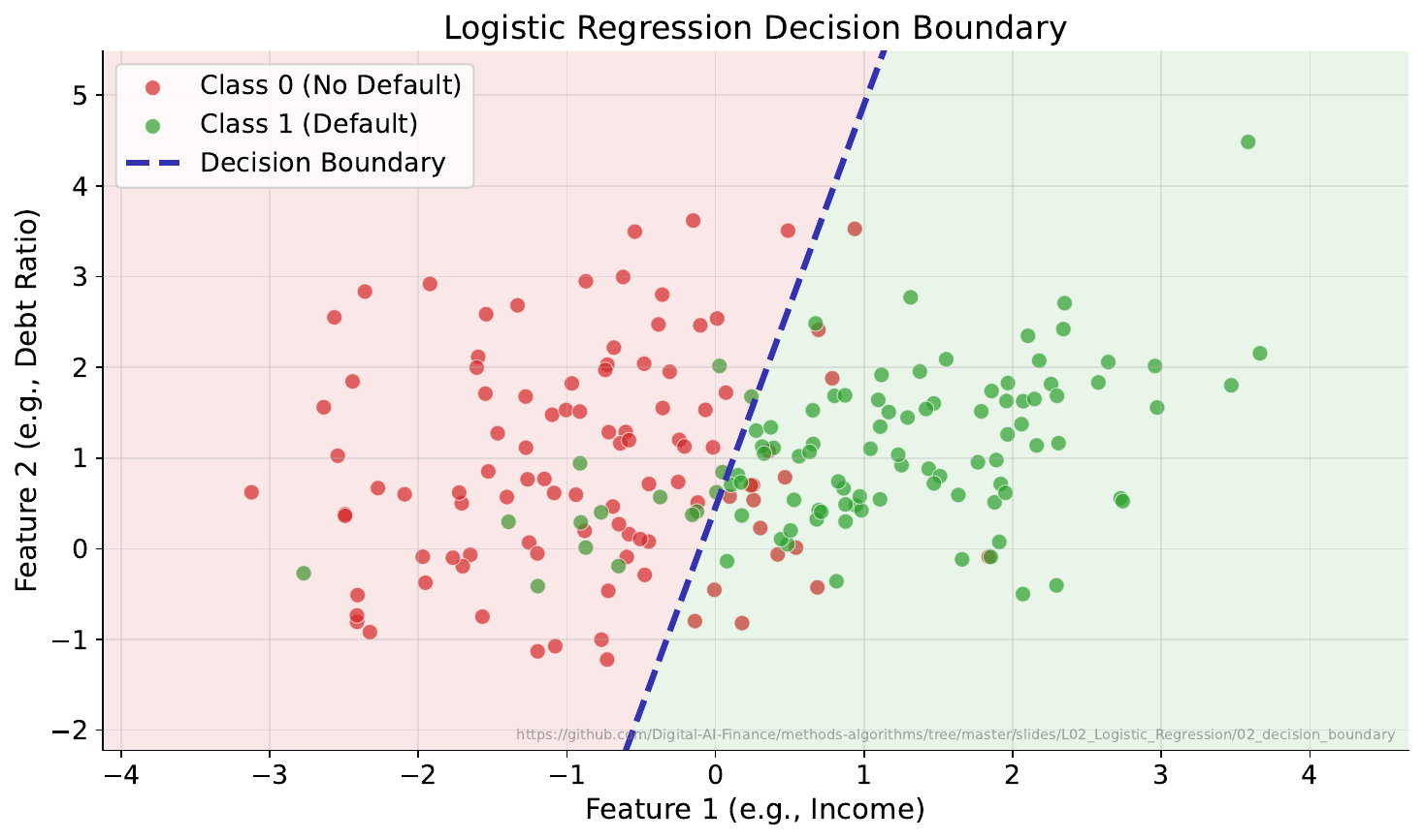
"Where Do You Draw the Line?"

Decision boundary separating two classes in feature space

Your Task

Where would you place a boundary to separate the two groups?
Can a straight line do it perfectly?
What about the points near the boundary -- how confident should the model be about those?

Reveal Solution

The decision boundary is where $P(\text{class}=1) = 0.5$. In 2D feature space, logistic regression draws a straight line (or hyperplane in higher dimensions). Points near the boundary have probabilities close to 0.5 -- the model is uncertain. Points far away have probabilities near 0 or 1.

Activity 4

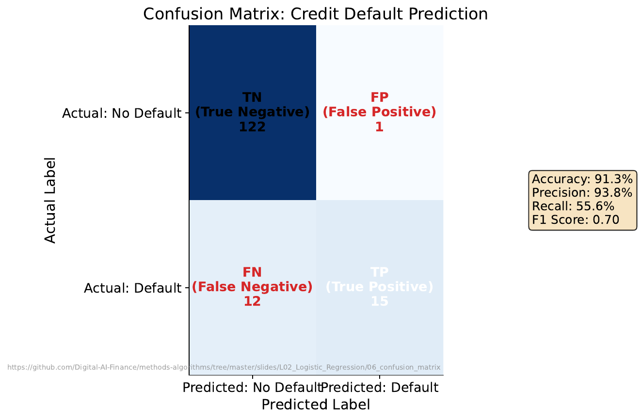
"The Confusion Table"

Confusion matrix showing true positives, false positives, true negatives, and false negatives

Your Task

In banking, which is worse: approving a bad loan (false positive) or rejecting a good customer (false negative)?
Count the errors in each category.
If you lower the approval threshold from 0.5 to 0.3, what changes?

Reveal Solution

The confusion matrix organizes predictions into TP, FP, TN, FN. Lowering the threshold approves more applicants -- increases true positives but also false positives. The trade-off between precision (how many approvals are correct) and recall (how many good customers you catch) is fundamental.

Activity 5

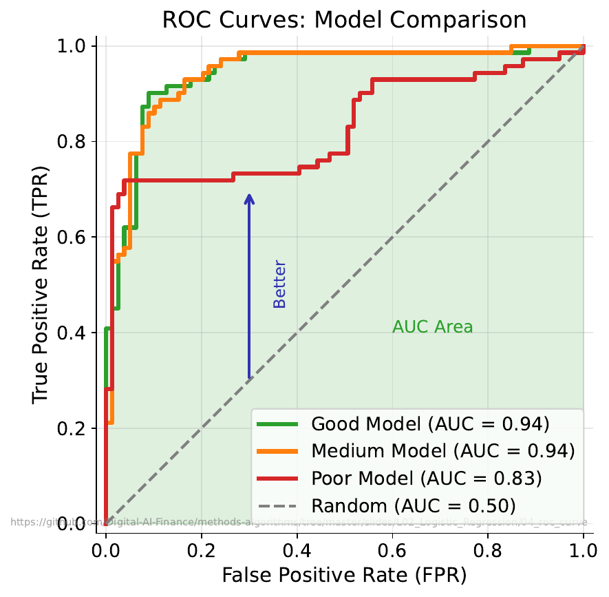
"Which Model Wins?"

ROC curves comparing model performance with diagonal random baseline

Your Task

What does the diagonal line represent?
Which curve is better and why?
Can a model be perfect -- what would that look like on this chart?

Reveal Solution

The diagonal is a random classifier (coin flip). The ROC curve plots True Positive Rate vs False Positive Rate at every threshold. A curve closer to the top-left is better. The AUC (Area Under Curve) summarizes performance: 0.5 = random, 1.0 = perfect. A perfect model reaches the top-left corner.

Activity 6

"Your Turn: Credit Scoring"

#	Income ($k)	Debt Ratio	Credit Score	Your Prediction
1	45	0.50	640	?
2	90	0.25	730	?
3	60	0.40	680	?
4	75	0.35	700	?
5	30	0.60	600	?
6	105	0.20	760	?

Your Task

Predict approve/deny for each applicant.
For each, rate your confidence from 0-100%.
Two applicants (#3 and #4) have similar incomes but might get different outcomes -- why?

Reveal Solution

Logistic regression combines all features: $P(\text{approve}) = \sigma(\beta_0 + \beta_1 \cdot \text{income} + \beta_2 \cdot \text{debt} + \beta_3 \cdot \text{score})$. Each feature contributes -- debt ratio might penalize #3 enough to shift the probability. Your confidence ratings are you intuitively doing what logistic regression formalizes!