Trading Macro Narratives
Evidence from LLM-Based Signals for Industry and Factor Portfolios
1University of Twente · 2Quoniam Asset Management
Abstract
We study whether directional macro-narrative scores extracted from news can be used to form cross-sectional signals for U.S. equity and factor portfolios. Using 65 evergreen narratives over 2004–2025, we estimate expanding-window narrative betas and combine them with weekly changes in narrative scores to construct two related strategies: a characteristics-weighted portfolio that ranks assets by exposure to current narrative shifts, and a narrative momentum portfolio that ranks narratives by their recent score trends. We compare a prompted large language model (LLM) sentiment score with a simpler bag-of-words (BoW) attention measure and with a non-text benchmark based on principal components from the FRED-MD macro panel. Across both asset universes considered, the LLM-based signals generate positive returns in both portfolio constructions, while the BoW baseline is generally weaker and the macro benchmark remains competitive. The evidence is most naturally interpreted as showing that directional narrative measures extracted from text can complement traditional macro signals, rather than as a stand-alone replacement. Overall, the results are encouraging but still provisional: economic magnitudes are moderate, performance is not uniform across specifications, and questions of turnover, trading costs, and broader implementability remain open.
Keywords. Narrative economics; macro themes; cross-sectional allocation; narrative betas; large language models; characteristics-weighted portfolios.
What this paper does, in five points
- Builds weekly directional sentiment scores for 65 evergreen macro narratives using a prompted LLM, and compares them against a bag-of-words attention baseline and against principal components from the FRED-MD macro panel.
- Estimates expanding-window narrative betas and constructs a characteristics-weighted (CW) portfolio that tilts toward assets with strong exposure to current narrative shifts.
- Constructs a complementary narrative-momentum strategy in the spirit of Lee et al. (2024), going long narratives with rising scores and short those with falling scores via beta-sorted mimicking portfolios.
- Finds that LLM signals produce positive Sharpe ratios in both constructions (~0.4–0.5), that the two strategies are weakly correlated and diversify each other (combined SR up to +0.65 on 49-industry), and that the McCracken PCA benchmark remains competitive particularly in slow-moving episodes.
- Reads the results as evidence of complementarity with traditional macro signals rather than replacement. Magnitudes are moderate; turnover, trading costs, and implementability remain open.
1. Introduction
Recent work in narrative economics argues that stories help propagate economic fluctuations and shape beliefs about spending, investing, and policy (Shiller, 2017). In parallel, the text-as-data literature has shown that economic and financial text can be turned into quantitative state variables that capture sentiment, attention, and risk perceptions (Gentzkow, Kelly, & Taddy, 2019; Tetlock, 2007; Loughran & McDonald, 2011). News-based measures have been used to track business-cycle conditions, policy uncertainty, and broader macroeconomic narratives (Baker, Bloom, & Davis, 2016; Bybee et al., 2024; Flynn & Sastry, 2024).
Within asset pricing, recent work has begun to map such narratives into tradable signals. Bhargava et al. (2023) show that narrative betas—sensitivities of returns to changes in narrative scores—can be linked to market- and firm-level returns, while Lee et al. (2024) document momentum in narrative attention. This literature suggests that narrative measures may contain information that is not fully summarized by standard factors and macro datasets, but it also leaves open a practical question: how should narratives be quantified for portfolio construction?
That question matters because different text models measure different objects. Count-based or similarity-based methods are often well suited to capturing attention or topic intensity, but they can struggle with direction and context. More flexible language models, by contrast, can be used to assign directional scores to the same underlying themes. In this paper, we do not treat these approaches as strict substitutes. Instead, we ask whether LLM-based directional narrative scores contain useful cross-sectional information beyond a simpler bag-of-words (BoW) attention measure and beyond a traditional macro benchmark based on FRED-MD principal components (McCracken & Ng, 2016).
To answer this question, we construct weekly signals for 65 evergreen macro narratives using news headlines from January 2004 to July 2025. For each narrative and asset, we estimate expanding-window narrative betas from weekly returns on weekly changes in narrative scores. We then study two related portfolio constructions. The first is a characteristics-weighted (CW) strategy that ranks assets by the product of their narrative beta and the recent change in the corresponding narrative score. The second is a narrative momentum strategy in the spirit of Lee et al. (2024), which forms narrative-mimicking portfolios and then goes long narratives with improving scores and short narratives with deteriorating scores. We apply both approaches to the 49 Fama–French industry portfolios and to Fama–French factor-spread portfolios augmented with momentum (FF5+Mom).
This design yields four main results. First, LLM-based directional scores produce positive CW returns and cleaner signal monotonicity than the BoW baseline in both asset universes, although the magnitudes are moderate rather than decisive. Second, narrative momentum offers additional evidence that the LLM scores contain information not captured well by the BoW measure, but the strength of this result depends on the exact implementation and is best interpreted cautiously. Third, a benchmark built from McCracken-style macro data remains competitive, especially in slower-moving episodes, while the LLM-based signals appear most useful in fast-changing post-2020 environments. Taken together, the results point more toward complementarity with traditional macro signals than toward outright replacement. Fourth, the CW and narrative momentum strategies load on different dimensions of the same underlying data and therefore diversify each other, even though they rely on the same narrative scores and estimated betas.
Our contribution is therefore narrower than a claim that LLMs “solve” narrative trading. The paper provides new evidence that directional narrative scores extracted from news can be used to form portfolio signals that differ meaningfully from both count-based textual measures and standard macro factors. At the same time, the results leave several important questions open, including turnover, trading costs, concentration in the mimicking portfolios, and the stability of the signals across specifications. We view the evidence as a proof of concept and as a starting point for a broader comparison between textual narrative measures and conventional macroeconomic state variables.
Relatedly, our CW and narrative-momentum exercises are meant to illuminate two complementary uses of the same narrative panel. The CW strategy asks which assets should respond most to current narrative shifts; narrative momentum asks which narratives are themselves trending. Their joint performance therefore matters less as a pursuit of a single headline Sharpe ratio than as evidence that narrative information can be organized along multiple economically distinct dimensions.
The remainder of the paper proceeds as follows. Section 2 describes the narrative, return, and macro datasets. Section 3 outlines the beta estimation and portfolio constructions. Section 4 presents the empirical results, and the appendix reports additional crisis and sensitivity analyses.
2. Data
2.1 Narrative Scores
We use 65 evergreen narratives drawn from the taxonomy of Bhargava et al. (2023), excluding three event-specific narratives (COVID-19, Trade War, Brexit) that are absent over significant portions of the sample. Each narrative belongs to one of seven thematic “reservoirs”: Corporate, US Macroeconomic, Global Macro & Geopolitics, Financial Markets & Instruments, Investment Strategies, Sectors & Industries, and Society.
For the BoW baseline, the daily narrative score \(\theta_{n,t}^{\text{BoW}}\) is the average cosine similarity between all headlines on day \(t\) and the centroid embedding of narrative \(n\), filtered for negative sentiment. This is an attention measure: it captures how prominently a narrative features in the news flow, without distinguishing the direction of sentiment. BoW scores are non-negative and unbounded, surging during crises as article counts rise.
For the LLM model, the daily score \(\theta_{n,t}^{\text{LLM}}\) is a sentiment measure obtained from structured LLM calls. Each day’s headlines are grouped by overarching theme and passed to a prompted LLM that assigns one of five ordinal sentiment labels per narrative—negative, mostly negative, can’t tell, mostly positive, positive—mapped to \(\{-2, -1, 0, +1, +2\}\). The prompt instructs the model to assess whether the tone towards each narrative implies improving or deteriorating conditions (e.g., for “Recession,” negative indicates worsening recession risk, not negative sentiment about recessions). This design means the LLM score is bounded, ordinal, and inherently directional—properties that fundamentally shape its behaviour in both the CW portfolio and narrative momentum frameworks. Table 1 summarises score statistics by reservoir.
| Reservoir | N | BoW \(\bar\theta\) | BoW \(\sigma\) | BoW AC(1) | LLM \(\bar\theta\) | LLM \(\sigma\) | LLM AC(1) | \(\rho_\ell\) | \(\rho_\Delta\) |
|---|---|---|---|---|---|---|---|---|---|
| Corporate | 10 | 1.10 | 0.84 | 0.51 | 0.04 | 0.48 | 0.26 | −0.09 | −0.07 |
| Financial Markets & Instruments | 9 | 10.14 | 5.50 | 0.63 | −0.13 | 0.55 | 0.20 | −0.07 | −0.13 |
| Global Macro & Geopolitics | 7 | 1.47 | 1.12 | 0.52 | −0.20 | 0.47 | 0.42 | −0.37 | −0.17 |
| Investment Strategies | 11 | 1.03 | 0.89 | 0.69 | 0.14 | 0.31 | 0.14 | 0.01 | −0.05 |
| Sectors & Industries | 5 | 0.89 | 0.79 | 0.41 | −0.05 | 0.48 | 0.37 | −0.29 | −0.14 |
| Society | 8 | 0.73 | 0.89 | 0.43 | −0.08 | 0.20 | 0.26 | −0.27 | −0.16 |
| US Macroeconomic | 15 | 12.14 | 7.49 | 0.45 | −0.40 | 0.69 | 0.39 | −0.15 | −0.03 |
Notes. \(N\) is the number of narratives in each reservoir. \(\bar\theta\) denotes the time-series mean of the weekly score. AC(1) is the first-order autocorrelation. \(\rho_\ell\) and \(\rho_\Delta\) are the cross-model correlations in levels and first differences, respectively.
A notable feature is that cross-model change correlations (\(\rho_\Delta\)) are negative across all reservoirs, ranging from −0.03 (US Macroeconomic) to −0.17 (Global Macro & Geopolitics). This suggests the two models respond to different aspects of narrative dynamics. Full narrative-level descriptives are omitted for brevity.
2.2 Industry Returns
We use value-weighted excess returns for the 49 Fama–French industry portfolios, obtained from Kenneth French’s data library. Daily returns are aggregated to weekly frequency by compounding. We also construct factor spread portfolios from the five Fama–French factors (MKT, SMB, HML, RMW, CMA) plus momentum (MOM). The sample runs from January 2004 through July 2025 (approximately 1,125 weekly observations).
2.3 McCracken PCA Macro-Factor Benchmark
As a non-textual benchmark, we use ten principal components extracted from the FRED-MD macroeconomic panel of McCracken and Ng (2016). FRED-MD comprises over 100 monthly U.S. macroeconomic time series—covering employment, industrial production, interest rates, prices, housing, and financial conditions—transformed to stationarity and reduced via PCA to ten factors (\(F_1, \ldots, F_{10}\)). We work with monthly first differences of these factors, yielding a panel of ten monthly macro-innovation series available from 1960 onward.
The McCracken benchmark applies the same signal-construction pipeline as the narrative models. Monthly expanding-window betas are estimated by regressing each asset’s monthly return on each factor change, using all data up to month \(t\) with a minimum window of 12 months. Because the FRED-MD panel begins decades before the narrative sample, the expanding window incorporates approximately 34 years of history by the start of our evaluation period in 2004, providing substantially more estimation data than the narrative betas (which begin in 2003). Monthly signals (\(\beta_{i,f,t}\times\Delta F_{f,t}\)) are forward-filled to weekly dates and then enter the same lagging, rank-scaling, and portfolio-construction steps described in Section 3.
This benchmark tests whether the cross-sectional information in narrative signals could be replicated by standard macroeconomic data. If the narrative signal merely proxies for macro-factor exposures, the McCracken PCA strategy should perform at least as well.
3. Methodology
The signal construction is inspired by the narrative-beta framework of Bhargava et al. (2023), adapted for industry-level cross-sectional analysis. We first describe the shared building blocks (3.1–3.2), then the two portfolio strategies that use them: the characteristics-weighted (CW) portfolio (3.3) and the narrative momentum strategy (3.4).
3.1 Weekly Aggregation and Beta Estimation
Daily narrative scores are resampled to weekly frequency by averaging within each Monday–Friday window:
where \(w\) indexes the calendar week. We then define weekly score changes as
Industry excess returns are compounded over the same window: \(R_{i,w} = \prod_{d \in w}(1 + r_{i,d}) - 1\). Weekend observations are excluded from all series.
For each narrative \(n\) and industry \(i\), we estimate an expanding-window univariate beta using all data up to week \(t\) (with a minimum of 52 weeks):
The beta \(\beta_{i,n,t}\) measures industry \(i\)’s contemporaneous sensitivity to weekly changes in narrative \(n\) as estimated at week \(t\), using an expanding window that incorporates all available history. Untabulated tests using a fixed 52-week rolling window lead to similar qualitative results.
3.2 Signal Construction
We define a general building block that underpins both the CW portfolio and the narrative momentum strategy. The smoothed score change for narrative \(n\) at horizon \(h\) weeks is:
Multiple lookbacks \(\mathcal{H} = \{h_1, h_2, h_3\}\) can be combined into a composite:
where \(\sigma_t^{(h)}\) is the cross-sectional standard deviation of the rolling-mean score change across all narratives at horizon \(h\). Each horizon’s rolling mean is divided by this dispersion before averaging, but not demeaned. This equalises the dispersion across horizons—shorter lookbacks have roughly twice the cross-sectional spread of longer ones—while preserving the cross-sectional mean, which carries economic information when the signal enters multiplicatively with \(\beta\). The single-week change \(\Delta\theta_{n,t}\) is the degenerate case \(\mathcal{H} = \{1\}\). Short lookbacks (1–12 weeks) capture high-frequency news flow and are natural for cross-sectional asset allocation (“which industries are moving now?”), while longer lookbacks (12–52 weeks) identify persistent narrative trends suited for cross-narrative selection (“which stories have sustained momentum?”). We specify the horizons used by each strategy in their respective sections below.
3.3 Characteristics-Weighted Portfolio
The CW signal for industry \(i\), narrative \(n\), week \(t\) is:
This captures both the direction and magnitude of the industry’s narrative exposure, scaled by recent narrative shifts. Because the signal enters multiplicatively with \(\beta\), the magnitude of \(\overline{\Delta\theta}\) carries economic information—a narrative undergoing a large shift should contribute more than one that is barely moving. We use a short-horizon composite \(\mathcal{H} = \{4, 8, 12\}\) weeks (\(\approx\) 1/2/3 months), which smooths over high-frequency noise while preserving the economic magnitude that the beta multiplier requires.
We apply a two-week lag to the raw signal (\(S_{i,n,t-2}\)) to ensure implementability and to accommodate the negative autocorrelation induced by differencing. The lagged signals are then rank-scaled cross-sectionally within each week:
where the rank-scaling assigns the most negative signal a weight of −2 and the most positive a weight of +2, with linear interpolation in between. The ranking is performed across all \((i, n)\) pairs on each date, ensuring cross-sectional comparability across the \(N_{\text{industries}} \times 65\) signal entries.
Industry excess returns are volatility-adjusted by dividing by rolling industry-level standard deviation (annualized):
The portfolio return on week \(t\) is the cross-sectional average of signal-weighted, volatility-adjusted returns:
where \(N\) is the total number of industry–narrative combinations. This is a characteristics-weighted portfolio in the sense of Brandt, Santa-Clara, and Valkanov (2009): the weight on each asset is a linear function of its narrative signal characteristic \(\tilde{S}_{i,n,t}\). By construction, the portfolio overweights industries with strong positive narrative signals and underweights those with negative signals.
3.4 Narrative Momentum Strategy
The CW framework exploits cross-asset variation in narrative betas: for a given narrative shift, which assets benefit most? A complementary question is which narratives are currently gaining or losing momentum, regardless of the specific assets they load on. Following Lee et al. (2024), we exploit momentum in narrative attention directly. Rather than weighting existing industry portfolios by narrative signals, this approach constructs narrative-mimicking portfolios—long-short equity portfolios that isolate the return associated with each narrative—and then goes long narratives with rising scores and short those with declining scores.
Mimicking portfolios
For each narrative \(n\) and week \(t\), we rank assets by their lagged expanding beta \(\beta_{i,n,t-1}\) and go long the asset with the highest beta and short the asset with the lowest beta. Each mimicking portfolio return is vol-scaled to 1% annualised volatility so that all narratives contribute equally to the spread portfolio. With 65 evergreen narratives and \(K=1\) assets per leg, this yields 65 mimicking portfolio return series per model and universe.
Narrative score momentum
We measure narrative momentum using the same rolling-mean operator \(\overline{\Delta\theta}_{n,t}^{(h)}\) defined in equation (2), evaluated at lookback \(M\) weeks:
At each week \(t\), narratives are ranked by \(\text{Mom}_{n,t-1}^{(M)}\) (lagged one week for implementability). The top \(J\) narratives are classified as rising and the bottom \(J\) as declining.
Spread portfolio
The spread portfolio return on week \(t\) is:
where \(r_{n,t}^{\text{mim}}\) is the vol-scaled mimicking portfolio return for narrative \(n\). For equity-line comparisons, the spread return is itself vol-normalised to 1% annualised.
We search over a grid of lookback horizons \(M \in \{2, 4, 6, 8, 10, 12, 16, 20, 26, 34, 39, 52\}\) weeks with \(J = 5\) narratives per leg (out of 65 evergreen). All betas are expanding-window estimates with a minimum of 52 weeks, consistent with the CW framework. As a benchmark, we apply the same momentum logic to the McCracken PCA factors, using monthly expanding betas (window = 12 months) forward-filled to weekly dates, monthly factor momentum forward-filled for weekly ranking, and \(J = 5\) factors per leg (out of 10).
Composite lookback signal
As in the CW strategy (equation 3), we combine multiple lookback horizons to avoid selecting a single \(M\). For narrative momentum, we use a long-horizon set \(\mathcal{H} = \{12, 26, 52\}\) weeks (roughly quarterly, semi-annual, and annual). As in the CW composite, each horizon’s rolling mean is cross-sectionally vol-scaled before averaging:
where \(\sigma_t^{(M)} = \operatorname{std}_n\!\bigl(\text{Mom}_{n,t}^{(M)}\bigr)\) is the cross-narrative standard deviation at week \(t\). This equalises horizon contributions—shorter lookbacks have roughly twice the cross-sectional dispersion of longer ones—while preserving the cross-narrative mean. Narratives are ranked by \(\text{Mom}_{n,t-1}^{\,\text{comp}}\) and assigned to rising (\(J = 5\)) and declining (\(J = 5\)) legs as in the single-lookback case. For the McCracken PCA benchmark, the analogous composite uses \(M \in \{3, 6, 12\}\) months.
4. Results
4.1 Signal-Weighted Portfolio Performance
Table 2 reports the performance of the characteristics-weighted (CW) strategy across two asset universes, alongside the BoW and McCracken PCA baselines and two further benchmarks: an equal-weighted average of vol-adjusted returns and a momentum-weighted strategy.
| Universe | Strategy | Ann. Ret | Vol | Sharpe | NW-\(t\) |
|---|---|---|---|---|---|
| 12-Ind | BoW | 0.0000 | 0.0009 | 0.04 | 0.19 |
| LLM-sentiment | 0.0009 | 0.0019 | 0.48 | 2.20 | |
| Avg Vol-Adj | −0.0005 | 0.0029 | −0.18 | −0.86 | |
| 12m Mom | 0.0013 | 0.0053 | 0.24 | 1.17 | |
| 49-Ind | BoW | 0.0000 | 0.0006 | 0.07 | 0.39 |
| LLM-sentiment | 0.0006 | 0.0013 | 0.48 | 2.20 | |
| Avg Vol-Adj | 0.0000 | 0.0029 | −0.02 | −0.07 | |
| 12m Mom | 0.0010 | 0.0039 | 0.25 | 1.24 | |
| FF5+Mom | BoW | −0.0002 | 0.0012 | −0.20 | −0.99 |
| LLM-sentiment | 0.0008 | 0.0021 | 0.39 | 1.77 | |
| Avg Vol-Adj | 0.0011 | 0.0050 | 0.22 | 1.01 | |
| 1m Mom | 0.0007 | 0.0060 | 0.12 | 0.62 | |
| 49-Ind | McCracken PCA | 0.0005 | 0.0014 | 0.37 | 1.70 |
| FF5+Mom | McCracken PCA | 0.0008 | 0.0023 | 0.33 | 1.62 |
Notes. Ann. Ret and Vol are annualized from weekly returns. Sharpe is the annualized Sharpe ratio. NW-\(t\) is the Newey–West \(t\)-statistic on the mean weekly return. Benchmarks: “Avg Vol-Adj” is the equal-weighted average of vol-adjusted asset returns; “12m Mom” (“1m Mom” for FF5+Mom) is a momentum CW strategy using 52-week (4-week) rolling mean returns as the signal.
LLM-sentiment generates positive returns across all universes, with Sharpe ratios of 0.48 (49-Ind) and 0.39 (FF5+Mom). BoW is flat on 49-Ind (SR 0.07) and negative on FF5+Mom, consistent with the composite smoothing washing out its high-frequency count spikes.
Figures 1 and 2 show cumulative returns across both universes, benchmarked against the equal-weighted average vol-adjusted return, a momentum CW strategy, and a McCracken PCA macro-factor CW portfolio. The McCracken benchmark applies the same CW framework using ten principal components extracted from the FRED-MD panel (McCracken & Ng, 2016) as factors: expanding betas are estimated at monthly frequency (from 1970 onward) and the resulting signals are forward-filled to weekly dates.
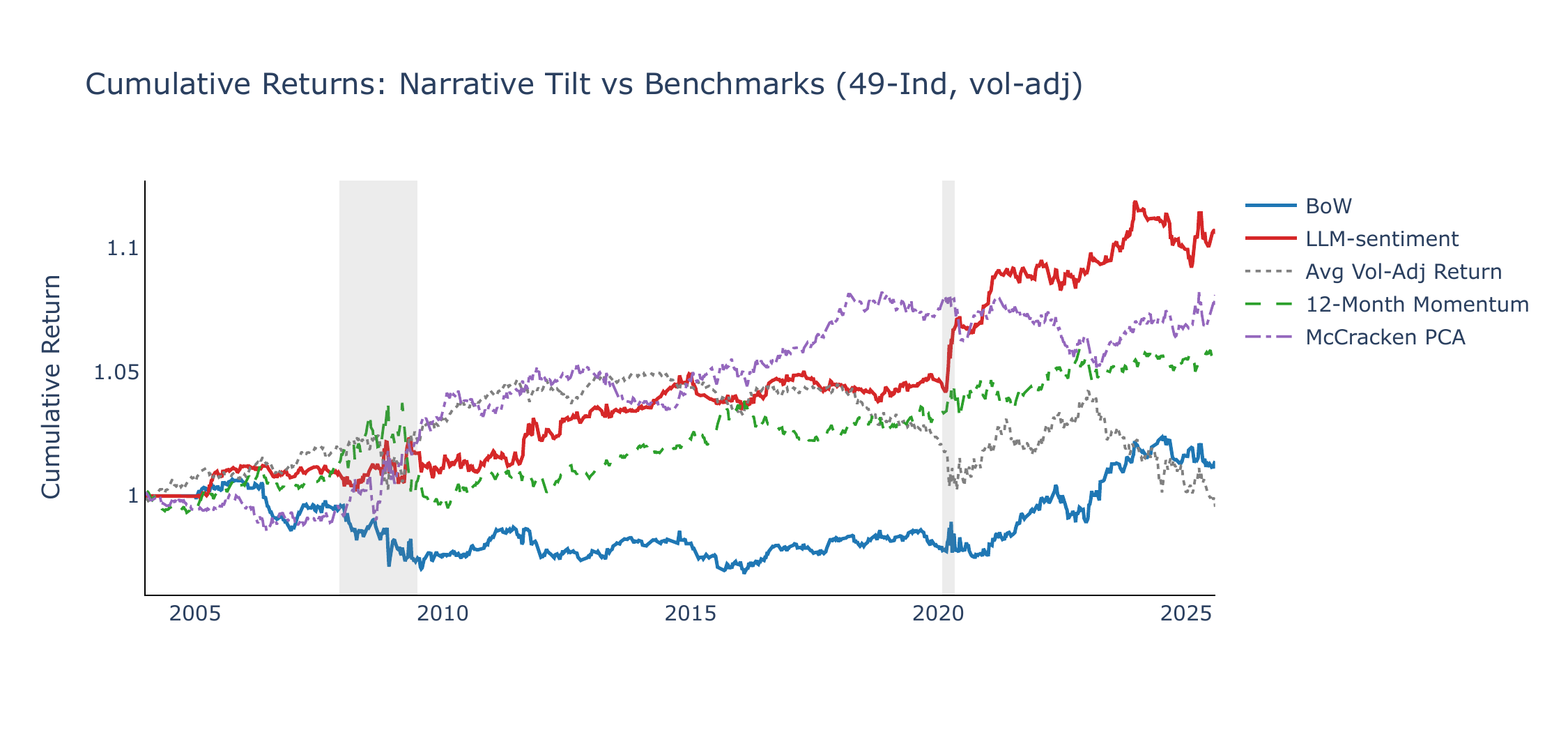
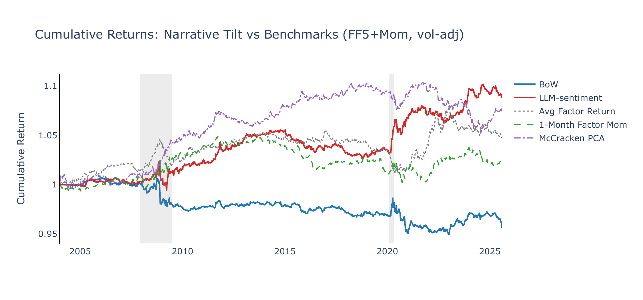
Across both universes, the LLM CW strategy outperforms the equal-weighted benchmark, which weakens notably after COVID. The McCracken PCA baseline is a meaningful comparator (Sharpe 0.37 on 49-Ind, 0.33 on FF5+Mom), outperforming both momentum and BoW despite benefiting from a substantially longer estimation history (expanding betas from 1970 vs. \(\sim\)2003 for narratives). LLM-sentiment modestly exceeds McCracken in both universes (0.48 vs. 0.37 and 0.39 vs. 0.33), but the comparison is best read as evidence of complementarity rather than dominance: the macro-factor signal is stronger in slower-moving episodes, whereas the LLM signal appears to adapt more quickly after 2020.
4.2 Signal Informativeness and Narrative Selection
A central question for the CW framework is which narrative signals carry economically meaningful information and whether informative signals can be identified ex ante. We address this from three angles: cross-sectional monotonicity (quintile sorts), thematic decomposition (narrative groups), and historical breakout filters.
Quintile analysis
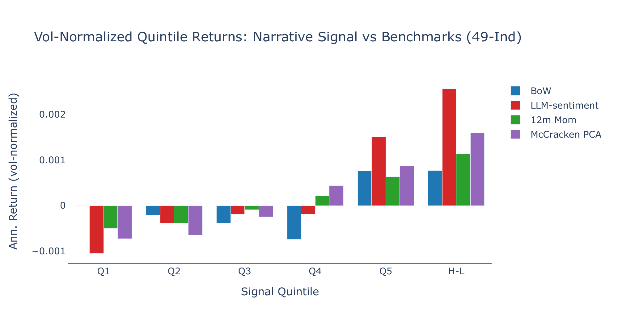
We sort industry–narrative–week observations into quintiles based on the lagged, rank-scaled signal \(\tilde{S}_{i,n,t}\) and compute average vol-adjusted returns within each quintile. Table 3 reports the results.
| Universe | Model | Q1 | Q2 | Q3 | Q4 | Q5 | H−L | H−L \(t\) | H−L SR |
|---|---|---|---|---|---|---|---|---|---|
| 12-Ind | BoW | −0.0006 | −0.0003 | −0.0006 | −0.0007 | −0.0003 | 0.0003 | 0.46 | 0.09 |
| LLM-sentiment | −0.0019 | −0.0004 | −0.0007 | −0.0003 | 0.0007 | 0.0026 | 2.28 | 0.49 | |
| 12m Mom | −0.0020 | −0.0014 | −0.0003 | −0.0001 | 0.0012 | 0.0033 | 1.20 | 0.25 | |
| 49-Ind | BoW | 0.0000 | −0.0001 | −0.0002 | −0.0003 | 0.0003 | 0.0003 | 0.86 | 0.16 |
| LLM-sentiment | −0.0008 | −0.0003 | −0.0001 | −0.0001 | 0.0012 | 0.0020 | 2.47 | 0.53 | |
| 12m Mom | −0.0010 | −0.0008 | −0.0002 | 0.0005 | 0.0013 | 0.0024 | 1.17 | 0.24 | |
| McCracken PCA | −0.0005 | −0.0005 | −0.0002 | 0.0003 | 0.0006 | 0.0012 | 1.55 | 0.33 |
Notes. Quintiles (Q1–Q5) are formed by sorting industry–narrative–week observations on the lagged, rank-scaled signal. H−L is the high-minus-low spread. The FF5+Mom universe reports tercile sorts (T1–T3) omitted here for brevity; see the PDF.
Both models exhibit a monotonically increasing pattern from Q1 to Q5 on the 49-industry universe. LLM-sentiment produces a statistically significant long–short spread (SR 0.53, \(t=2.47\)), while BoW and McCracken PCA are weaker (SR 0.16 and 0.33 respectively). Figure 3 visualizes the return pattern.
Which narrative themes matter?
The CW portfolio aggregates signals from all 65 narratives. To understand which themes drive performance, we group narratives into six thematic clusters: Crisis & Stress (5 narratives; Recession, Risk, Market Crash, Bankruptcy, US Growth Slowdown); Policy Response (5; Federal Reserve, Interest Rates, Treasury Bonds, Fiscal, Money); Macro Fundamentals (8; Business Cycles, GDP, Inflation, Labor Market, Housing Market, US Growth, Personal Consumption, Personal Finance); Financial System (9; Commercial Banking, Investment Banking, Financing, Money Market, Liquidity, Government & Corporate Debt, Derivative Securities, Fund & Asset Management, FX); Global (7; China Growth, Emerging Markets, Global Growth, Globalization, International Trade, International Conflicts, International Organizations); and Other (31; Investment Strategies, Society, Sectors & Industries, plus remaining corporate and market-structure narratives). Table 4 decomposes the CW return into additive contributions from each group over the full sample and during two crisis subperiods. For each date, the rank-scaling is performed globally across all \(N_{\text{assets}} \times 65\) signals, so group contributions sum exactly to the total.
| Universe | Group | Full | GFC | COVID | |||
|---|---|---|---|---|---|---|---|
| BoW | LLM | BoW | LLM | BoW | LLM | ||
| 49-Ind | Crisis | 0.2 | 0.4 | 0.4 | 1.5 | 10.5 | −0.9 |
| Policy | −0.1 | 0.2 | −3.5 | −3.4 | −2.4 | 6.1 | |
| Macro Fund. | −0.4 | 1.0 | −3.5 | 2.0 | −2.7 | 22.6 | |
| Fin. System | 0.4 | 1.0 | −0.1 | 2.1 | −3.4 | 11.8 | |
| Global | 0.0 | 0.7 | 0.7 | 0.7 | 0.5 | 10.5 | |
| Other | 0.4 | 3.1 | −1.8 | 3.4 | 11.4 | 60.7 | |
| Total | 0.4 | 6.4 | −7.9 | 6.4 | 13.9 | 110.7 | |
| FF5+Mom | Crisis | 0.2 | 0.5 | 2.1 | 0.5 | 21.5 | −1.0 |
| Policy | −0.8 | 0.4 | −6.7 | −3.2 | 3.5 | 4.1 | |
| Macro Fund. | 0.1 | 1.1 | 2.7 | 5.4 | 1.9 | 39.3 | |
| Fin. System | −0.4 | 1.3 | 0.5 | −0.1 | −5.9 | 30.5 | |
| Global | −0.3 | 0.7 | 0.8 | 3.4 | 0.0 | 17.7 | |
| Other | −1.2 | 4.0 | −15.9 | 7.8 | 44.9 | 117.0 | |
| Total | −2.4 | 8.1 | −16.4 | 13.8 | 66.0 | 207.6 | |
Notes. Each entry is the annualised CW return contribution (in basis points) from the narrative group, using the globally rank-scaled signal \(\tilde{S} \in [-2,+2]\). Contributions are additive across groups for each (Universe, Model, Period). Full = Jan 2004–Jul 2025; GFC = Dec 2007–Jun 2009; COVID = Feb–Apr 2020.
Over the full sample, the decomposition reveals that no single narrative group dominates. On 49-Ind, the LLM total of +6.4 bps is distributed across all groups, with “Other” (+3.1 bps) and “Macro Fundamentals” / “Financial System” (+1.0 bps each) contributing the most. On FF5+Mom the pattern is similar: LLM total +8.1 bps, with “Other” (+4.0 bps) the largest contributor. The BoW baseline generates lower full-sample contributions across all groups, consistent with its weaker aggregate Sharpe ratio. Importantly, the informativeness is spread across themes rather than concentrated in a few crisis-related narratives—suggesting that the signal captures a broad channel of cross-sectional information.
During the GFC, both models generate mildly negative total returns (−4 to −8 bps on 49-Ind). The “Crisis & Stress” narratives—the most directly relevant group—contribute at most ±1 bp, confirming that neither model generates large enough \(\beta \times \Delta\theta\) signals to dominate the ranking during a slow-burn crisis.
During COVID, the pattern changes materially. LLM returns are broad-based: “Other” (factor, strategy, and sentiment narratives) contributes +60.7 bps on 49-Ind and +117 bps on FF5+Mom, while the Financial System adds +11.8 bps and +30.5 bps. BoW earns its COVID returns primarily through “Crisis & Stress” (+10.5 bps on 49-Ind), where the sharp attention surge generates large \(\Delta\theta\) signals. Policy Response narratives show a telling asymmetry: the LLM captures the unprecedented Fed intervention (+6.1 bps on 49-Ind) while BoW’s policy signal is negative (−2.4 bps). The LLM’s COVID advantage thus stems not from better crisis detection but from capturing broad-based sentiment shifts across many non-crisis themes during the rapid recovery.
Extreme signal filter
We further test whether concentrating on narrative signals that break out of their own history improves informativeness. A percentile breakout filter retains, per (asset, narrative), only observations where the lagged signal exceeds its expanding 80th percentile or falls below its 20th percentile. The surviving signals are re-rank-scaled to \([-2, +2]\) per date and used to form a filtered CW portfolio. For comparison, the same filter is applied to the McCracken PCA baseline. We focus on this filter for brevity.
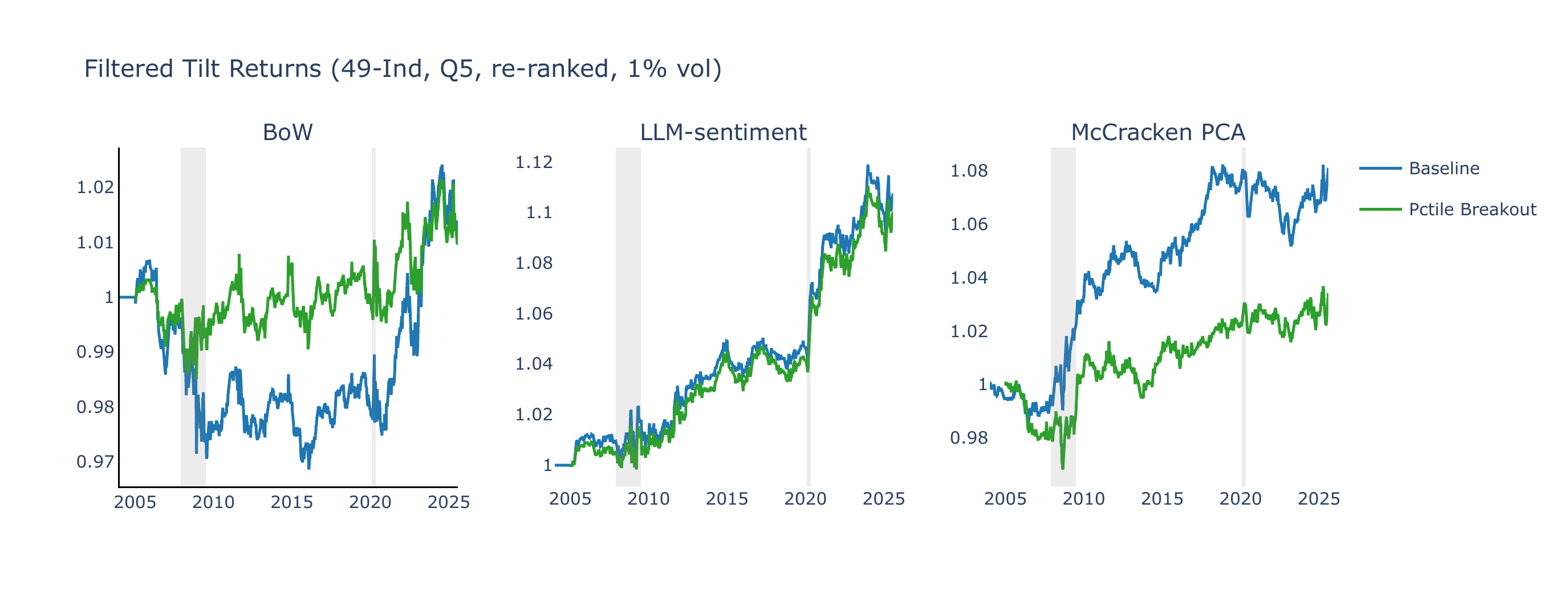
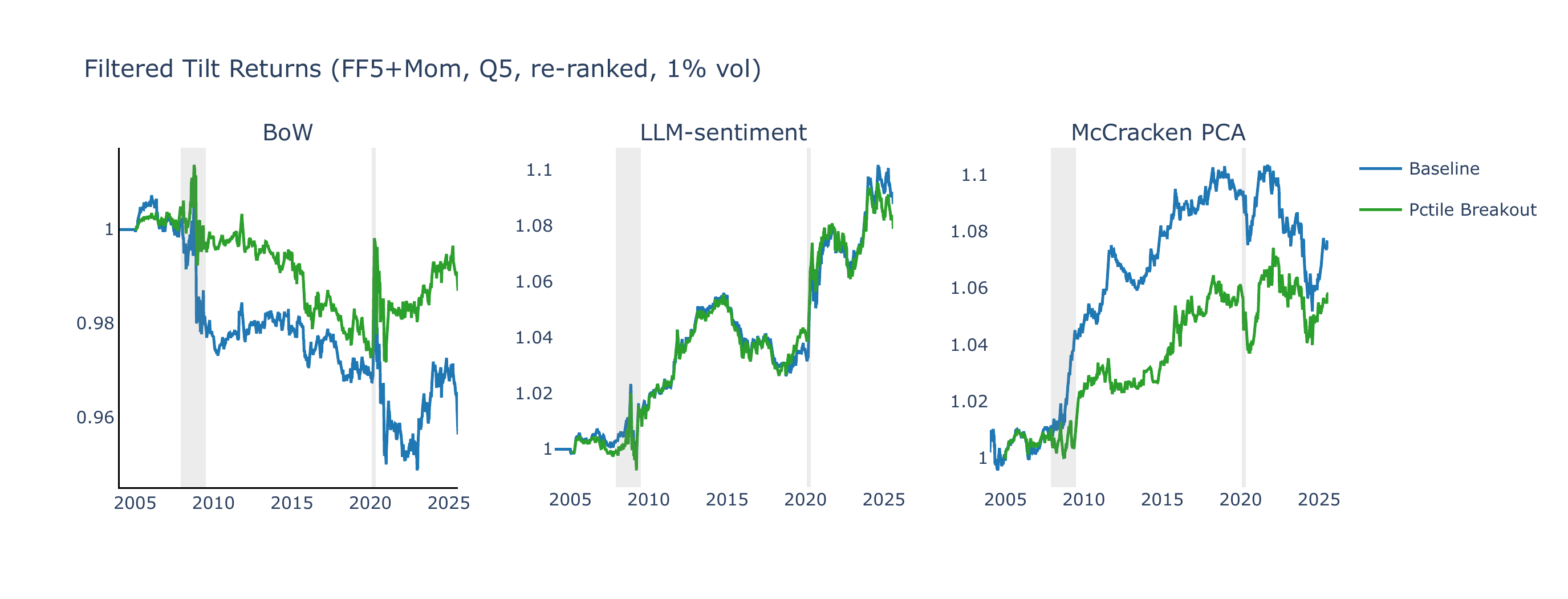
For narrative models, the percentile-breakout filter leaves the results broadly unchanged: concentrating the portfolio on signals that break out of their historical range retains most of the full-sample Sharpe ratio while roughly halving the number of active positions. On the 49-industry universe, LLM-sentiment percentile-breakout delivers a CW Sharpe of 0.47 (vs. 0.48 baseline). The McCracken PCA panel reveals a different pattern: the percentile filter weakens McCracken performance, and the Z-score filter performs poorly. One interpretation is that a narrative breaking out of its historical range can reflect a genuine shift in market attention, whereas extreme values of a PCA macro factor may more often reflect estimation noise or atypical months in the slowly updating FRED-MD panel.
Taken together, these three exercises provide supportive rather than definitive evidence on signal informativeness. The LLM signal is more monotonic in quintile sorts, its contributions are spread across several narrative themes, and concentrating on historical breakouts does not materially weaken performance. These patterns are consistent with the view that the narrative CW signal contains cross-sectional information not fully captured by the benchmarks considered here.
Crisis regimes
The bounded nature of LLM sentiment scores implies a structural regime dependence: during protracted crises such as the GFC, weekly score changes \(\Delta\theta \approx 0\) for crisis narratives, leaving both the CW and narrative momentum strategies with little to rank on (both LLM lines are flat during 2008–09 in Figure 11). By contrast, the McCracken PCA baseline—driven by slow-moving monthly macro data—generates strong positive returns during the GFC (Sharpe ratios of 0.82 and 1.43 on 49-Ind and FF5+Mom, respectively) but reacts more slowly during the rapid COVID shock, where narrative CW portfolios perform better. This difference again points to complementarity rather than a clear pecking order: bounded directional sentiment can lose resolution when narratives remain uniformly negative, whereas monthly macro data can be slow to update when regimes shift abruptly. Appendix A provides a detailed cyclical-versus-defensive decomposition during the GFC, a crash-versus-junk-rally subperiod analysis, and a discussion of the differencing asymmetry between BoW and LLM models.
A double sort on narrative signal × momentum suggests that the LLM-sentiment signal is largely orthogonal to industry momentum, whereas the BoW baseline is more closely subsumed by it.
4.3 Narrative Momentum
The contrast between BoW and LLM-sentiment narrative momentum is closely related to the differencing asymmetry discussed in Appendix A. BoW scores are unbounded counts that exhibit sharp spikes and mean reversion: high \(\Delta\theta\) today often predicts negative \(\Delta\theta\) tomorrow as the count reverts, producing an implicit contrarian force that works against momentum. LLM sentiment, by contrast, is bounded and more persistent: rising sentiment can signal improving conditions for a narrative, and the rolling average smooths over the noise in weekly changes that rendered the single-period \(\beta \times \Delta\theta\) signal less informative during crises. Appendix B shows that the more favorable LLM results are fairly stable across lookback horizons and the number of narratives per leg, but more sensitive to the concentration choice \(K\) in the mimicking portfolios.
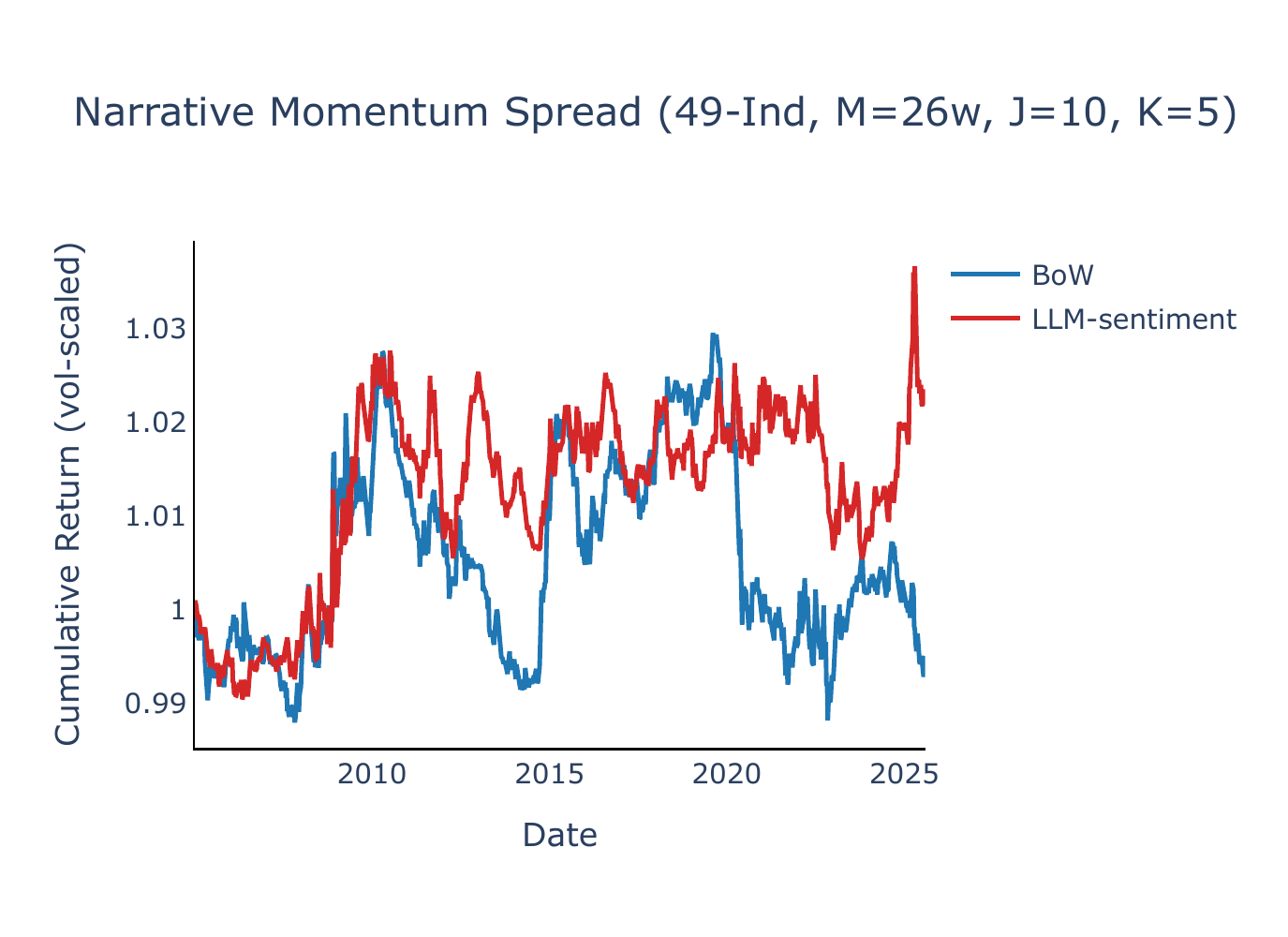
Headline equity lines
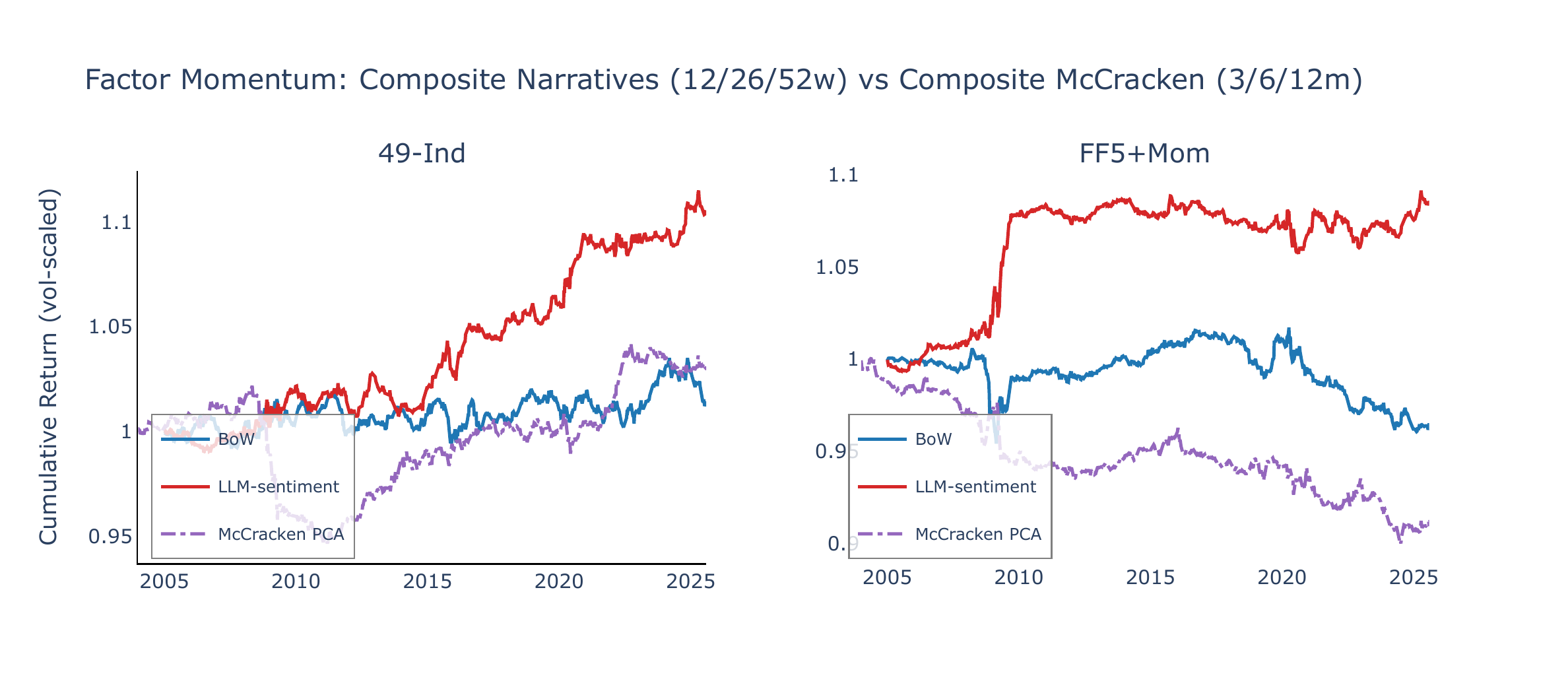
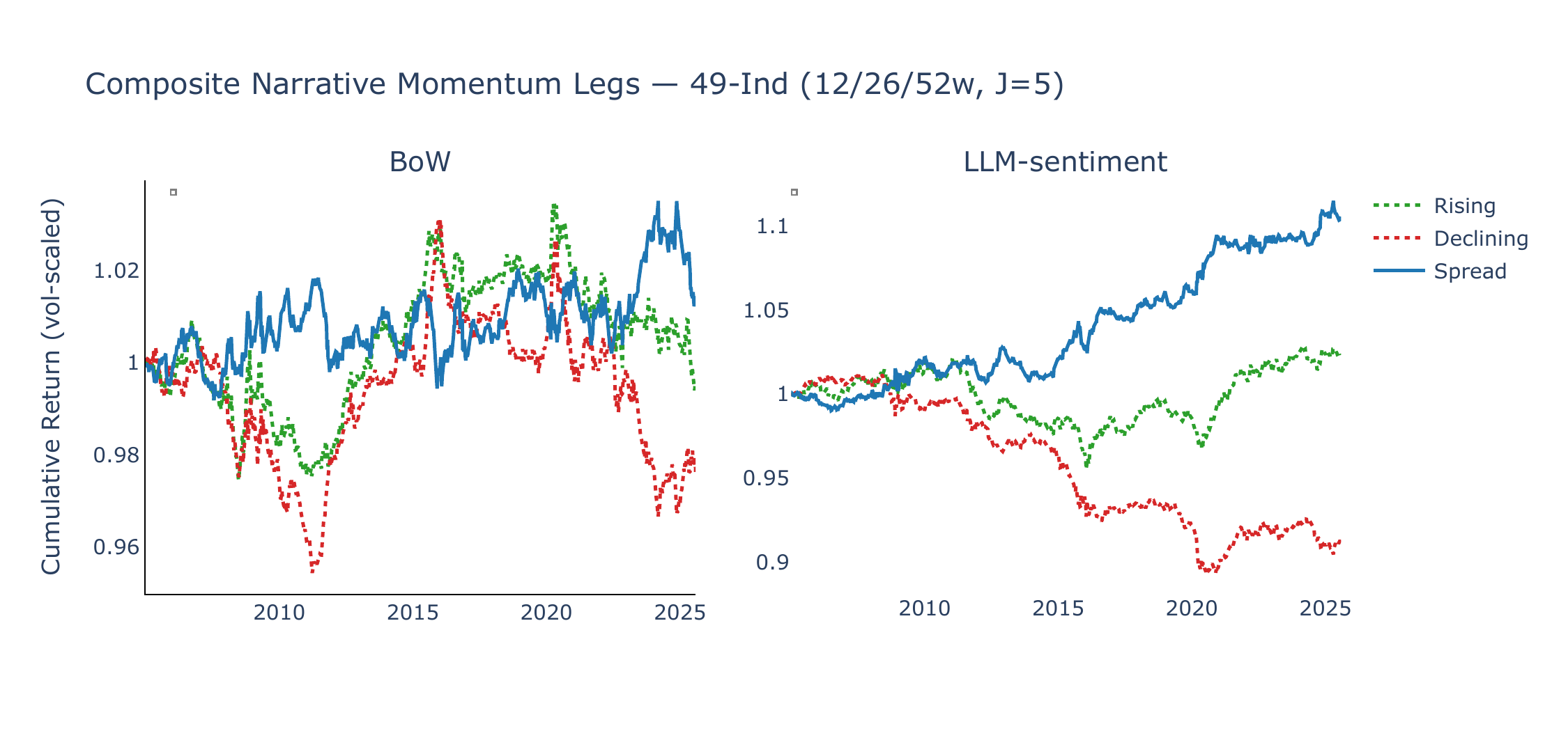
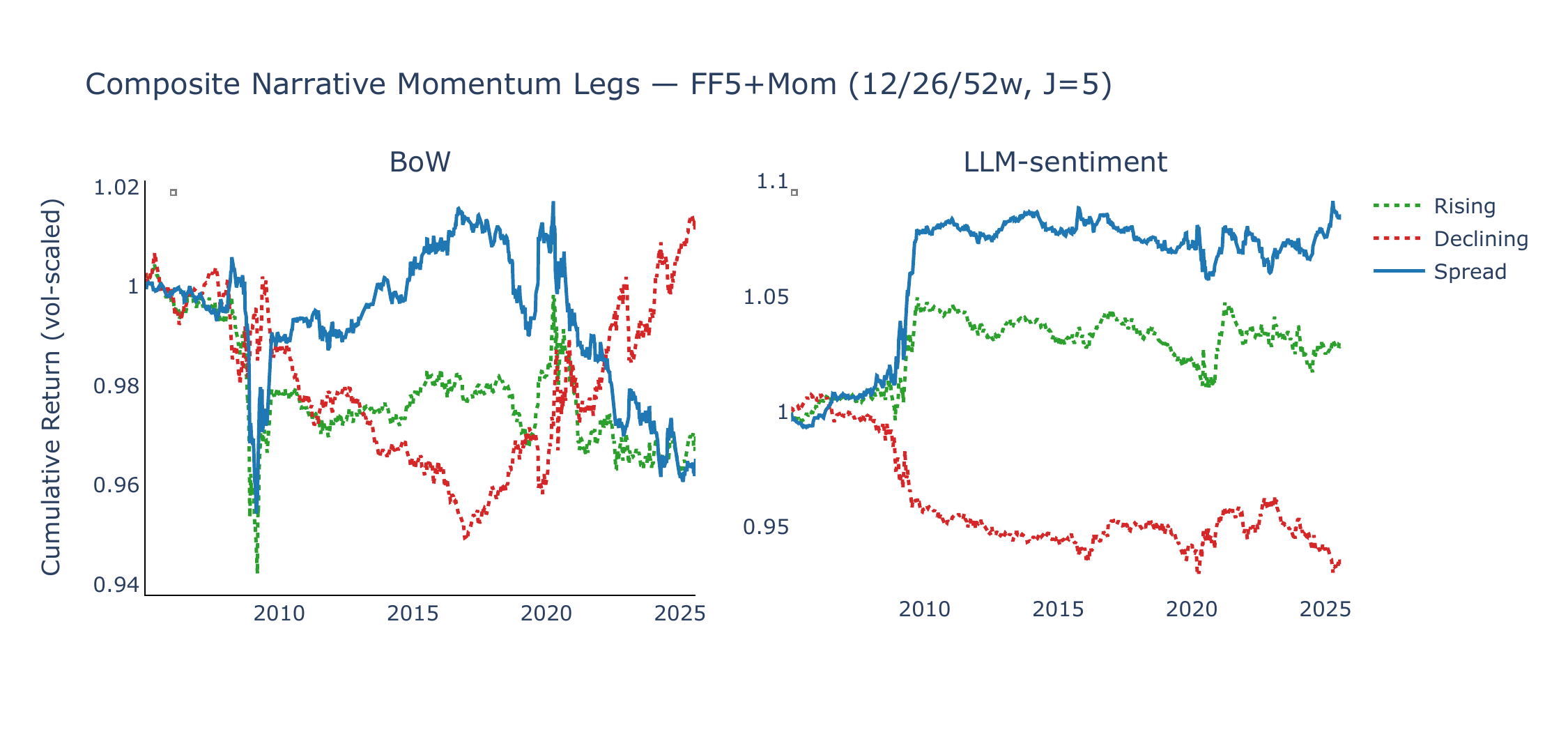
Figure 6 shows the cumulative spread returns under the composite signal (12/26/52w lookback average, \(J = 5\)), vol-normalised to 1% annualised, alongside a composite McCracken PCA factor momentum strategy (3/6/12-month lookback average, \(J = 5\) factors per leg). LLM-sentiment narrative momentum generates positive average returns and upward drift in both universes, while BoW momentum is flat or declining. McCracken PCA composite momentum is likewise flat or negative (SR = +0.15 on 49-Ind, −0.43 on FF5+Mom), suggesting that momentum in monthly macro-factor changes does not translate well into cross-sectional asset return predictability at our horizons.
Controlling for price momentum
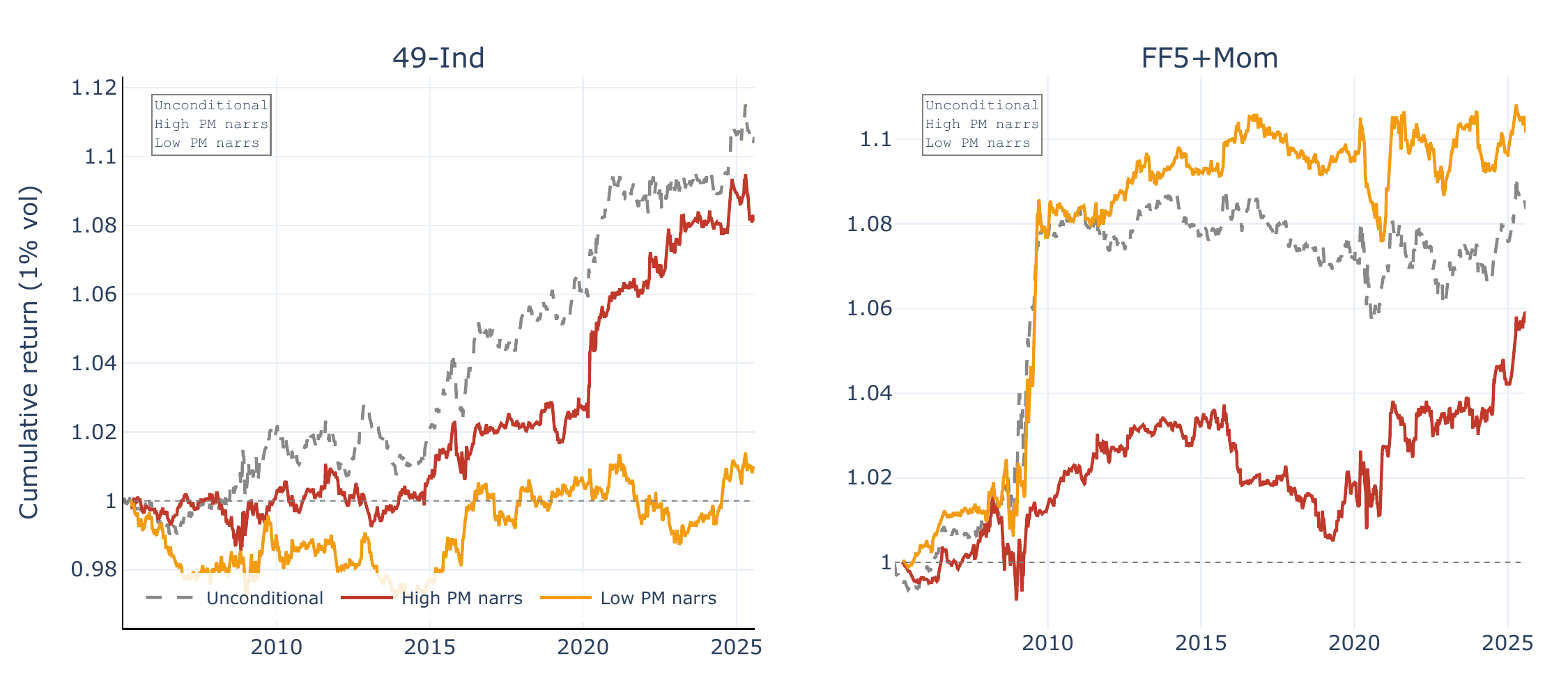
A natural concern is that narrative momentum may simply proxy for return momentum in the underlying mimicking portfolios: if a narrative’s mimicking portfolio has recently earned high returns, that same narrative is likely to exhibit rising scores (positive news begets attention), and the narrative momentum spread would merely repackage a price-momentum effect. To test this, we perform a double sort at each date. Narratives are first median-split by their mimicking portfolio’s cumulative 26-week return, producing a High PM and a Low PM group of roughly 32–33 narratives each. Within each group, narratives are then ranked by the composite score momentum signal, and the top/bottom \(J = 5\) form the rising and declining legs. Figure 7 plots the resulting vol-scaled equity lines for LLM-sentiment, and Table 5 reports summary statistics for both models.
The results reveal an instructive asymmetry across asset universes. For the 49-industry universe, narrative momentum is concentrated among narratives whose mimicking portfolios have recently performed well (High PM: SR = +0.39, \(t = 1.94\); Low PM: SR = +0.06, \(t = 0.29\)). This suggests that, at the industry level, narrative score momentum and price momentum partially reinforce each other: rising media attention for an industry tends to coincide with positive mimicking-portfolio returns, and the combined signal is stronger than either component alone. For the FF5+Mom factor universe, the pattern reverses: narrative momentum is stronger among low-price-momentum narratives (Low PM: SR = +0.48, \(t = 1.84\); High PM: SR = +0.27, \(t = 1.35\)). Here, narrative momentum captures factor-return predictability that is largely orthogonal to—and, if anything, contrarian to—recent mimicking-portfolio performance.
Taken together, these results make it unlikely that narrative momentum is merely repackaged price momentum. The industry-level correlation between the two signals is consistent with a common underlying driver (attention begets both media coverage and trading), but the factor-level reversal suggests that the narrative signal contains information that is at least partly distinct from recent mimicking-portfolio returns. For BoW, price-momentum conditioning has negligible impact: both High PM and Low PM spreads are near zero, consistent with the weak BoW narrative momentum performance documented above.
| Model | Universe | Group | SR | NW-\(t\) | Ann. Ret (%) | Ann. Vol (%) |
|---|---|---|---|---|---|---|
| BoW | 49-Ind | High PM | +0.02 | +0.07 | +0.01 | 0.60 |
| Low PM | −0.04 | −0.17 | −0.02 | 0.54 | ||
| Unconditional | +0.07 | +0.34 | +0.05 | 0.66 | ||
| FF5+Mom | High PM | +0.02 | +0.10 | +0.01 | 0.52 | |
| Low PM | −0.67 | −2.76 | −0.37 | 0.56 | ||
| Unconditional | −0.17 | −0.69 | −0.12 | 0.72 | ||
| LLM-sentiment | 49-Ind | High PM | +0.39 | +1.93 | +0.27 | 0.69 |
| Low PM | +0.05 | +0.27 | +0.03 | 0.60 | ||
| Unconditional | +0.49 | +2.37 | +0.37 | 0.76 | ||
| FF5+Mom | High PM | +0.28 | +1.39 | +0.19 | 0.67 | |
| Low PM | +0.48 | +1.83 | +0.27 | 0.56 | ||
| Unconditional | +0.39 | +1.71 | +0.29 | 0.75 |
Notes. Narratives are median-split by 26-week mimicking-portfolio cumulative return (High/Low PM), then sorted by composite score momentum within each group. “Unconditional” is the baseline composite spread without PM conditioning. SR is annualised Sharpe ratio; NW-\(t\) is the Newey–West \(t\)-statistic on mean weekly returns.
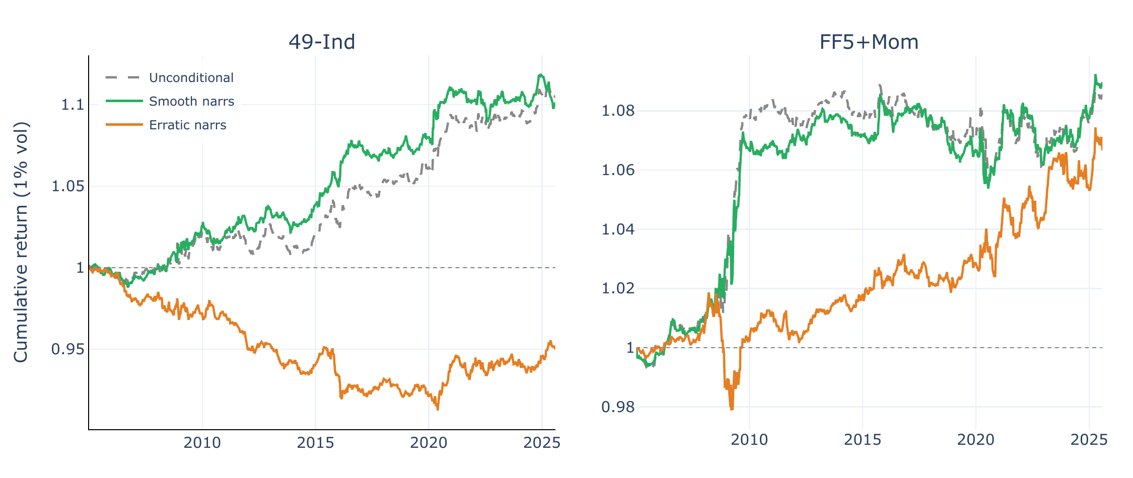
Information smoothness
Da, Gurun, and Warachka (2014) show that gradual information arrival generates stronger momentum because investors under-react to smooth trends more than to discrete jumps—the “frog in the pan” effect. Following Lee et al. (2024), we test whether narrative momentum is stronger for smoothly trending narratives. At each date, we compute an expanding-window smoothness metric for each narrative’s score changes: \(|\overline{\Delta\theta}| / \sigma(\Delta\theta)\), where the mean and standard deviation are computed with an expanding window (minimum 52 weeks). High smoothness indicates a narrative whose score changes consistently in one direction; low smoothness indicates erratic fluctuations. Narratives are median-split into Smooth and Erratic groups, and the composite narrative momentum spread is computed within each group. Figure 8 shows that the LLM-sentiment momentum spread is more concentrated among smoothly trending narratives, which is suggestive of the frog-in-the-pan hypothesis: gradual sentiment shifts may attract less investor attention and therefore be more slowly impounded into prices.
Rising vs. declining legs
Figures 9 and 10 decompose the composite spread into its rising (long) and declining (short) legs. For LLM-sentiment, the rising leg contributes most of the positive return in both universes, indicating that the strategy appears to profit primarily from identifying narratives whose improving sentiment is associated with favourable asset returns, rather than from shorting narratives with deteriorating sentiment. BoW exhibits a mirror-image pattern where the declining leg occasionally generates positive returns (betting against mean-reverting attention spikes), but these gains are offset by the rising leg’s losses.
Summary
| Model | Universe | Ann. Ret | Ann. Vol | Sharpe | NW-\(t\) |
|---|---|---|---|---|---|
| BoW | 49-Ind | +0.000 | 0.007 | +0.07 | +0.34 |
| FF5+Mom | −0.001 | 0.007 | −0.17 | −0.69 | |
| LLM-sentiment | 49-Ind | +0.004 | 0.008 | +0.49 | +2.37 |
| FF5+Mom | +0.003 | 0.007 | +0.39 | +1.70 | |
| McCracken PCA | 49-Ind | +0.001 | 0.008 | +0.15 | +0.70 |
| FF5+Mom | −0.003 | 0.007 | −0.43 | −1.95 |
Notes. Narrative models use the composite 12/26/52-week lookback signal (cross-sectionally vol-scaled and equal-weighted) with \(J = 5\) narratives per leg and \(K = 1\) assets per mimicking portfolio. McCracken PCA uses the composite 3/6/12-month lookback.
The narrative momentum results support the broader conclusion that directional narrative scores can be useful beyond the contemporaneous CW signal. Relative to the BoW baseline, the LLM scores generate smoother and more persistent score changes that are more compatible with a momentum construction. At the same time, the economic magnitudes are moderate and, as Appendix B shows, the strategy is not equally robust to all implementation choices. Narrative momentum should therefore be read as complementary evidence rather than as a stand-alone result.
4.4 Two Dimensions of Narrative Information
The CW portfolio and narrative momentum strategies exploit different dimensions of the same underlying data: the former ranks assets by their narrative exposure (\(\beta \times \Delta\theta\)), the latter ranks narratives by their score trend. Both are built on expanding betas estimated from the same narrative–asset panel, yet they produce nearly uncorrelated weekly return streams. Table 7 reports pairwise correlations and Sharpe ratios for a simple equal-weighted combination.
| Model | Universe | CW SR | NarrMom SR | Corr | Combo SR | Combo NW-\(t\) |
|---|---|---|---|---|---|---|
| BoW | 49-Ind | 0.07 | 0.08 | 0.07 | 0.10 | 0.50 |
| FF5+Mom | −0.21 | −0.17 | 0.28 | −0.23 | −1.05 | |
| LLM-sentiment | 49-Ind | 0.49 | 0.49 | 0.14 | 0.65 | 3.01 |
| FF5+Mom | 0.40 | 0.39 | 0.21 | 0.51 | 2.27 | |
| McCracken PCA | 49-Ind | 0.37 | 0.26 | 0.15 | 0.41 | 1.93 |
| FF5+Mom | 0.36 | 0.00 | 0.22 | 0.23 | 1.12 |
Notes. Each component is vol-scaled to 1% annualised before combining with equal (50/50) weights. Corr is the Pearson correlation of weekly returns. NW-\(t\) is the Newey–West \(t\)-statistic on the mean weekly return of the combination. McCracken PCA uses monthly FRED-MD factors with expanding betas from 1970; narrative momentum uses the composite 3/6/12-month lookback.
For LLM-sentiment, the two strategies exhibit only weak positive correlation (\(\rho = +0.14\) on 49-Ind, +0.21 on FF5+Mom) yet individually achieve comparable Sharpe ratios (\(\sim\)0.4–0.5). The equal-weighted combination therefore achieves a higher Sharpe ratio than either component alone: SR +0.65 (\(t = 3.01\)) on 49-Ind and SR +0.51 (\(t = 2.27\)) on FF5+Mom. The McCracken PCA baseline, despite its strong CW performance, produces flat or negative narrative momentum (SR +0.15 on 49-Ind, −0.43 on FF5+Mom), limiting its combination potential. Figures 11 and 12 show the cumulative equity lines.
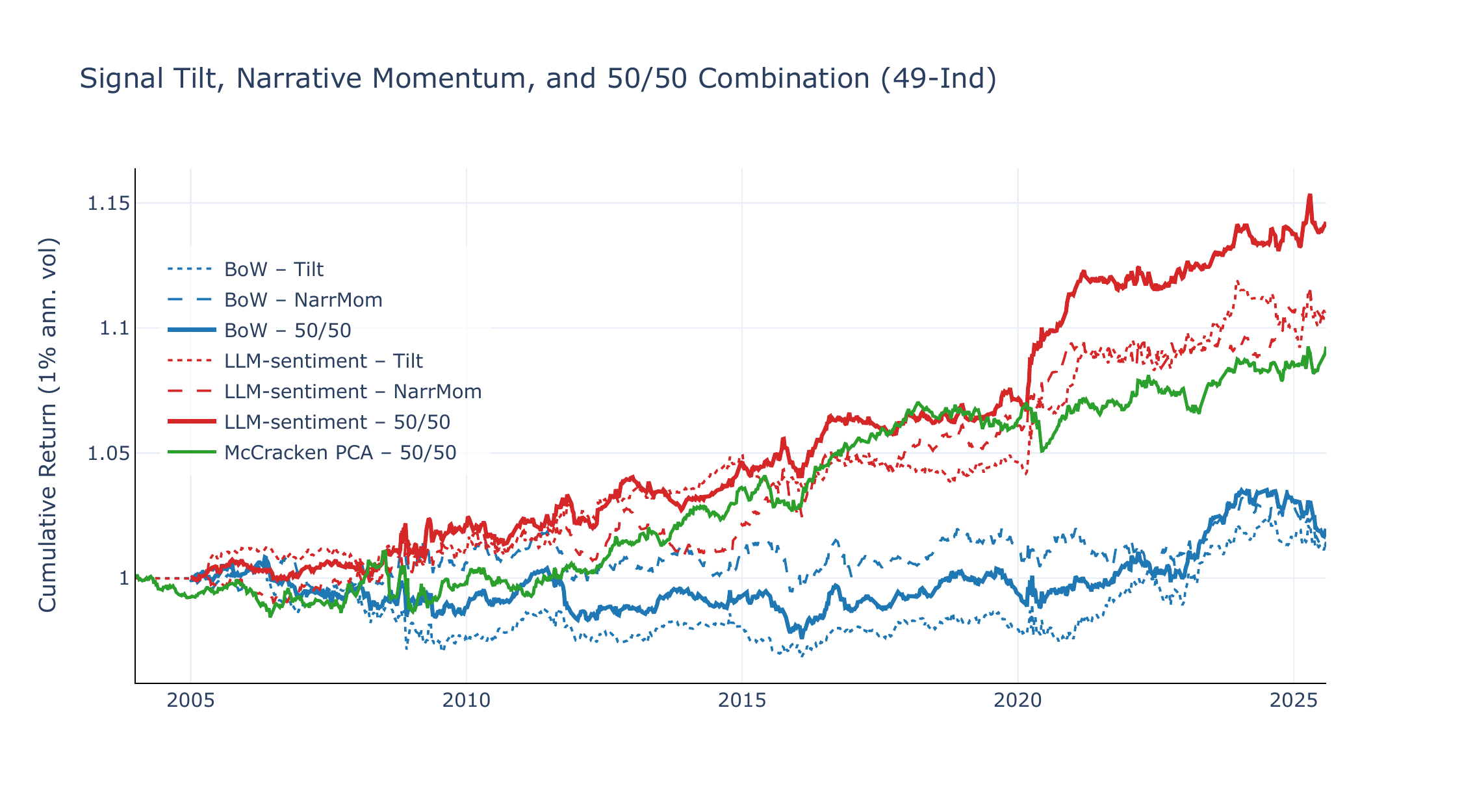
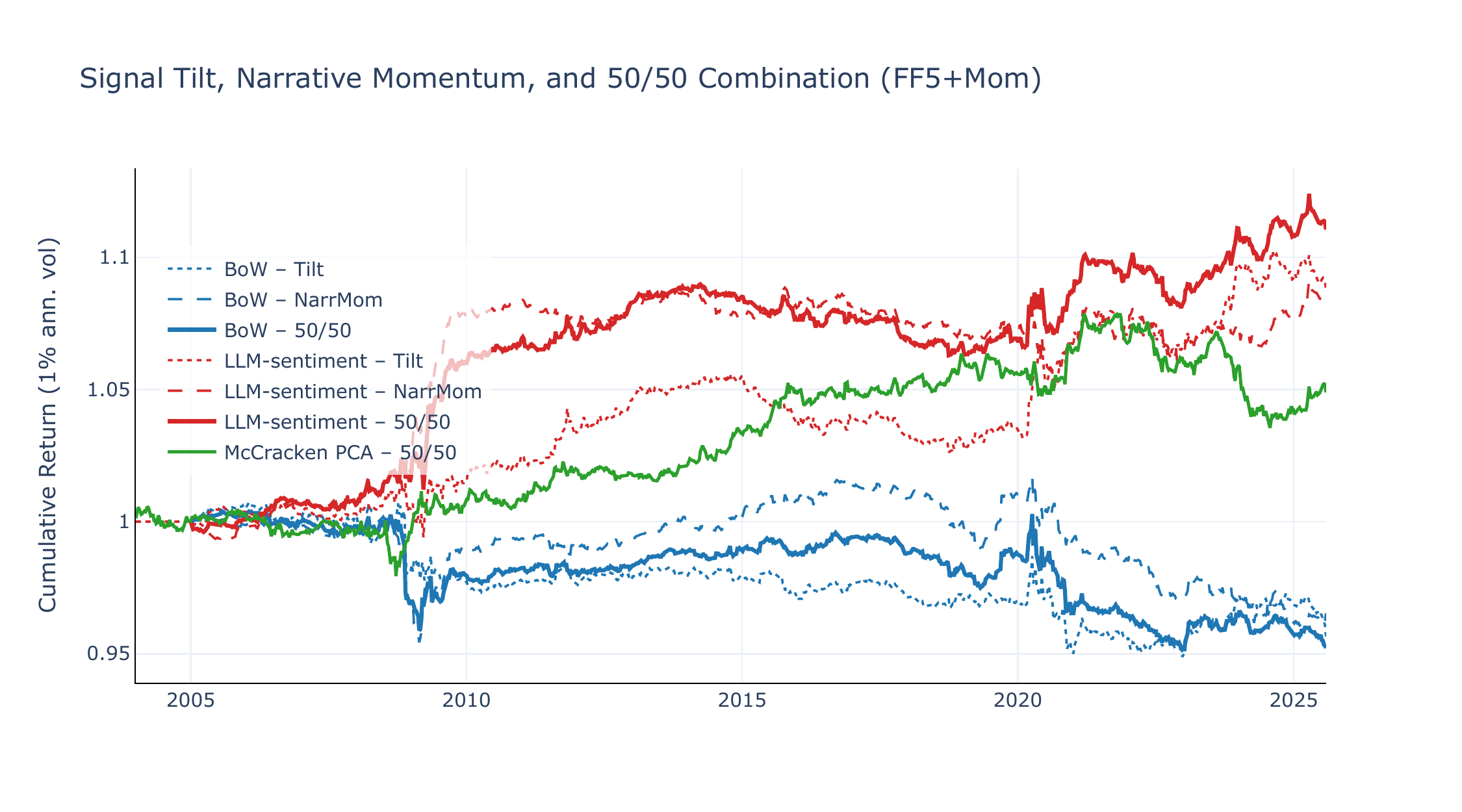
The low correlation is consistent with the economic interpretation: the CW portfolio responds to which assets are sensitive to current narrative shifts (cross-asset variation in \(\beta\)), while narrative momentum responds to which narratives are trending (cross-narrative variation in \(\overline{\Delta\theta}\)). The modest positive correlation (\(\rho \approx 0.1\)–0.2) likely reflects the shared use of expanding betas and the composite \(\overline{\Delta\theta}\) operator, but the two strategies’ distinct aggregation dimensions—across assets vs. across narratives—ensure substantial diversification. A positive LLM CW return requires both a strong narrative shift and high beta dispersion across assets; a positive narrative momentum return requires persistent score trends and beta-sorted mimicking portfolios that correctly isolate the narrative’s asset-level impact. These are distinct conditions that need not coincide, explaining why the two return streams diversify effectively.
For BoW, the combination offers no improvement: narrative momentum is flat or negative, so the combination inherits the CW portfolio’s modest Sharpe ratio on 49-Ind and degrades on FF5+Mom. The McCracken PCA benchmark illustrates a similar limitation from the opposite direction: its CW strategy performs competitively (Section 4), but the absence of meaningful factor momentum means that the combination cannot improve upon the CW return alone. Among the models considered here, only the LLM specification generates positive average returns in both dimensions, allowing the 50/50 combination to improve on either leg by itself. This is consistent with, though not conclusive proof of, the idea that directional narrative scores contain multiple layers of information that can be organized through complementary portfolio constructions.
5. Conclusion
This paper studies whether macro narratives extracted from news can be converted into useful cross-sectional portfolio signals. Across industry and factor-spread portfolios, LLM-based directional scores tend to produce cleaner signal sorts and better average performance than a simpler BoW attention measure, and the same scores can also be used in a narrative-momentum construction. At the same time, the evidence is better described as encouraging than conclusive. Return premia are moderate, the momentum results are somewhat sensitive to implementation choices, and a non-text macro benchmark based on FRED-MD principal components remains a meaningful competitor.
The main message is therefore one of complementarity. Text-based directional narrative measures appear to capture information that is not fully summarized by count-based textual measures or by standard McCracken-style macro factors. This distinction is especially visible when the news flow changes quickly across narratives, whereas during slow-moving or uniformly negative stress episodes the bounded LLM scores can lose discriminatory power. In that sense, narratives and conventional macro state variables seem to emphasize different parts of the economic environment.
Several limitations are important. The paper does not yet address turnover or transaction costs in a way that would support a strong implementability claim. The narrative-mimicking portfolios are concentrated in some specifications, and the sensitivity analysis shows that some design choices matter materially. More generally, the comparison between the LLM and BoW approaches should be read as a comparison between two practically relevant ways of quantifying narratives, not as a clean horse race that isolates model architecture alone.
These limitations also suggest the next steps. A natural extension is to study implementability explicitly, including costs, turnover, alternative holding periods, and broader portfolio constraints. It would also be useful to compare directional narrative scores to richer macro benchmarks, to explore alternative scoring schemes that retain information in prolonged crisis regimes, and to test whether the results survive in other asset classes and geographies. On balance, the paper offers new evidence that narrative-based signals deserve a place alongside traditional macro information in cross-sectional allocation, even if they are not yet a stand-alone solution.
Appendix A. Crisis Analysis
The bounded nature of LLM sentiment scores implies a structural regime-dependence: during protracted crises, weekly score changes \(\Delta\theta \approx 0\) for crisis narratives, rendering both the CW and narrative momentum strategies uninformative. We examine two crises that represent opposite extremes: the GFC (December 2007 to June 2009), a protracted, fundamentals-driven downturn lasting eighteen months; and COVID (February to April 2020), a sharp three-month shock followed by an unprecedented monetary impulse and rapid recovery.
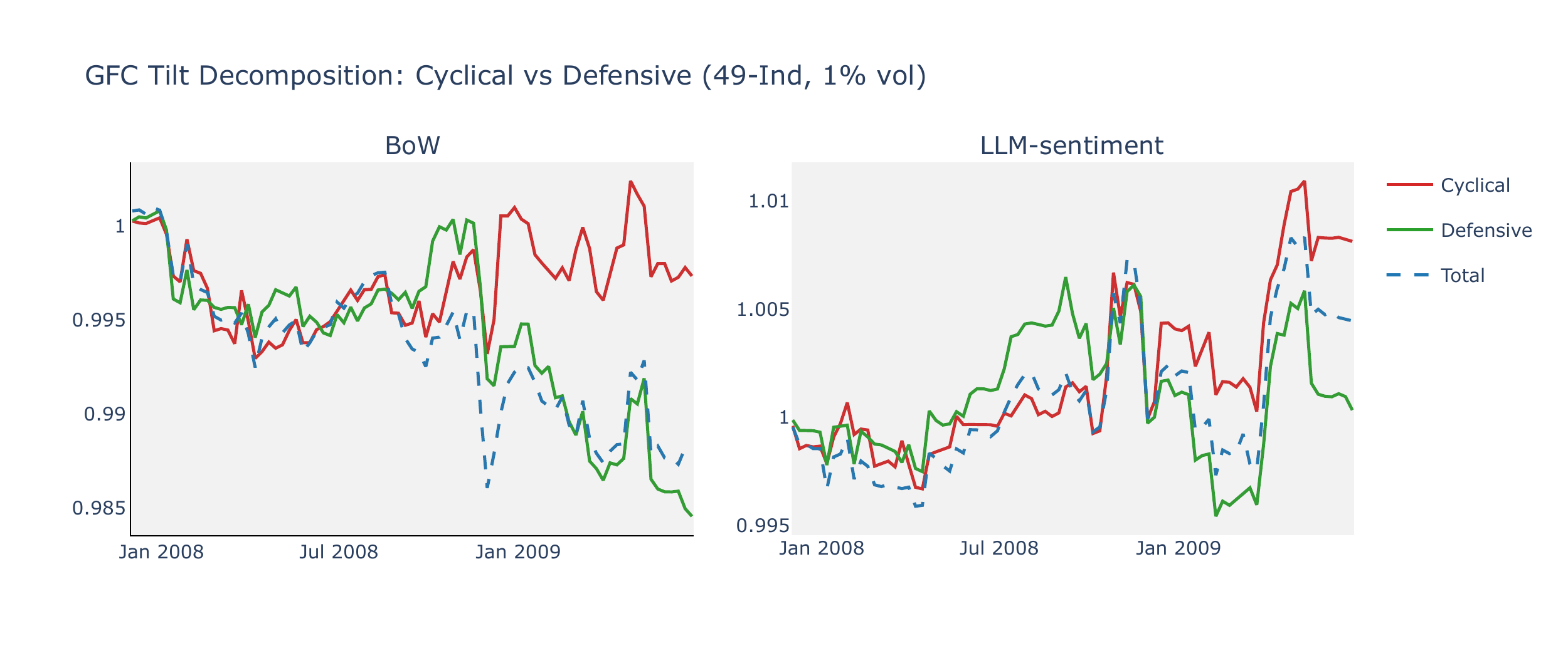
Cyclical vs defensive decomposition (49-Ind)
We classify eight unambiguously cyclical industries (Autos, Steel, Cnstr, Coal, Mines, Txtls, BldMt, Mach) and seven defensive industries (Food, Beer, Smoke, Drugs, Util, Hshld, MedEq), with the remaining 34 labelled “Other.” Table A1 decomposes the GFC-period CW return into contributions from each group.
| Model | Group | Avg Signal | Ann. Ret | Contribution | Share |
|---|---|---|---|---|---|
| BoW | Cyclical | 0.0151 | −0.0005 | −0.0004 | 0.52 |
| Defensive | −0.0140 | 0.0058 | −0.0024 | 3.00 | |
| Other | −0.0007 | 0.0001 | −0.0006 | 0.70 | |
| LLM-sentiment | Cyclical | −0.0034 | −0.0005 | 0.0027 | 4.22 |
| Defensive | 0.0068 | 0.0058 | 0.0001 | 0.21 | |
| Other | −0.0006 | 0.0001 | 0.0003 | 0.41 |
Notes. Avg Signal is the mean rank-scaled signal weight \(\tilde{S} \in [-2,+2]\), averaged across all (industry, narrative) pairs within the group and across GFC weeks. Ann. Ret is the annualized vol-adjusted return, averaged across industries within the group. Contribution is the group’s annualized CW return contribution (rank-scaled signal × vol-adjusted return). Share is the fraction of total CW return attributable to the group.
Several features of the decomposition merit comment. First, the LLM-sentiment cyclical contribution is positive (+22 bps annualised) and larger than BoW’s (+17 bps), despite the LLM’s mildly long-cyclical signal being the “wrong” crisis direction. Because \(\Delta\theta \approx 0\) for crisis narratives, the LLM CW portfolio does not short cyclicals during the drawdown—but equally does not miss the junk rally of March–June 2009, when the most beaten-down cyclical industries snap back aggressively while defensives lag. Second, defensive contributions are negative for both models—even BoW’s correctly signed long-defensive signal (\(\bar{S}=+0.002\)) yields −24 bps. This reflects the cross-sectional reversal characteristic of junk rallies: once the crisis troughs, capital rotates out of quality and defensive names into high-beta cyclicals, unwinding the protective gains accumulated during the drawdown. Over the full eighteen-month window it was difficult to earn positive defensive CW returns regardless of signal direction. The LLM’s total GFC shortfall relative to BoW therefore originates primarily from the defensive leg (−42 bps vs. −24 bps) rather than cyclicals, where the LLM’s flat crisis signal is partially self-correcting.
Crash versus junk rally
Splitting the GFC into the drawdown (December 2007 to March 2009, 67 weeks) and the subsequent junk rally (March to June 2009, 16 weeks) reveals that both models react to the regime change—though through different channels and with different effectiveness. Table A2 reports group-level signals and contributions for each subperiod.
| Model | Group | Crash (Dec 07–Mar 09) | Junk Rally (Mar–Jun 09) | Δ Signal | ||
|---|---|---|---|---|---|---|
| Avg Signal | Contribution | Avg Signal | Contribution | |||
| BoW | Cyclical | −0.013 | +0.001 | +0.039 | +0.006 | +0.052 |
| Defensive | +0.011 | −0.004 | −0.039 | +0.004 | −0.051 | |
| LLM-sentiment | Cyclical | −0.001 | +0.002 | +0.035 | +0.001 | +0.035 |
| Defensive | −0.001 | −0.004 | −0.053 | −0.003 | −0.053 | |
Notes. The GFC is split at March 9, 2009 (S&P 500 trough). Avg Signal is the mean rank-scaled weight \(\tilde{S} \in [-2,+2]\) averaged across industries, narratives, and weeks within the subperiod. Contribution is the annualised CW return contribution (\(\tilde{S} \times r^{\text{va}}\)). During the crash cyclicals return −1.2% ann. and defensives +1.4% ann.; during the rally these reverse to +4.6% and −2.6%.
The BoW model flips completely: from short-cyclical / long-defensive during the crash (\(\bar{S}_{\text{cyc}} = -0.013\), \(\bar{S}_{\text{def}} = +0.011\)) to long-cyclical / short-defensive during the rally (+0.039 and −0.039 respectively). The mechanism is straightforward—as crisis article counts decline from their peak, weekly changes \(\Delta\theta\) turn negative, and the \(\beta \times \Delta\theta\) signal reverses sign. The BoW model effectively reads “crisis abating” from falling narrative scores. This reversal is profitable: cyclical contributions swing from +1 bp (crash) to +57 bps (rally), while the defensive leg moves from −39 bps to +40 bps. Even during the crash, however, BoW’s long-defensive signal yields a negative contribution (−39 bps), indicating that the signal strengthened too late to capture the initial flight to quality.
The LLM-sentiment model also shifts into a long-cyclical / short-defensive posture during the rally (\(\bar{S}_{\text{cyc}} = +0.035\), \(\bar{S}_{\text{def}} = -0.053\)), from near-zero signals during the crash. The shift magnitude is comparable to BoW, but the channel differs: crisis narrative signals (Recession, Risk, Market Crash) remain flat for the LLM throughout both subperiods, because bounded sentiment scores generate negligible \(\Delta\theta\) regardless of the direction of change. Instead, the LLM reacts through non-crisis narratives—most notably “Business Cycles,” whose average sentiment improves from −1.72 during the crash to −0.69 during the rally, a shift of over one full point on the five-point scale. This improvement generates positive \(\Delta\theta\) that the cross-sectional ranking translates into a cyclical overweight. The LLM’s rally-phase contributions are, however, smaller and less clean than BoW’s: cyclical gains are modest (+14 bps) and the defensive leg remains negative (−34 bps), suggesting that the sentiment-based signal, while directionally correct, lacks the magnitude that BoW’s count-based reversal delivers.
FF5+Mom factor universe
We apply the same decomposition to the factor spread universe, classifying SMB and HML as cyclical factors (small and value spreads compress in downturns), RMW and CMA as defensive factors (profitability and conservative investment spreads are more stable), and Mom as procyclical.
| Model | Group | Factors | Avg Signal | Ann. Ret | Contribution | Share |
|---|---|---|---|---|---|---|
| BoW | Cyclical | SMB, HML | 0.0132 | 0.0019 | −0.0016 | 1.00 |
| Defensive | RMW, CMA | −0.0097 | 0.0072 | −0.0017 | 1.01 | |
| Procyclical | Mom | −0.0070 | −0.0102 | −0.0016 | 0.98 | |
| LLM-sentiment | Cyclical | SMB, HML | 0.0231 | 0.0019 | 0.0013 | 0.97 |
| Defensive | RMW, CMA | 0.0045 | 0.0072 | −0.0009 | −0.62 | |
| Procyclical | Mom | −0.0552 | −0.0102 | 0.0060 | 4.32 |
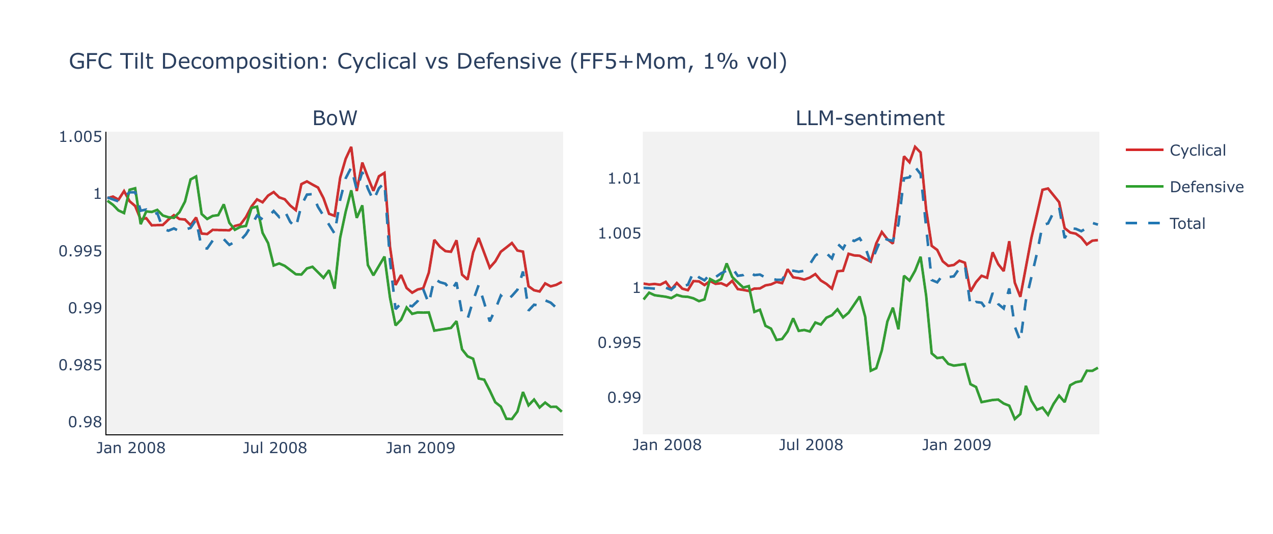
Signed narratives and the interpretation of raw betas
An important caveat applies to the interpretation of individual narrative betas, particularly for the LLM model. Many of the 65 narratives carry an inherent directional connotation—“Recession,” “Risk,” and “Market Crash” are intrinsically negative themes, while “Profitability” or “Smart Beta” are intrinsically positive. For the BoW model, the score measures attention (cosine similarity to a narrative centroid), and the beta captures how an asset’s return co-moves with changes in attention to that theme. For the LLM model, the score already incorporates sentiment direction: a persistently negative narrative like “Recession” will typically receive a negative LLM score regardless of whether conditions are improving or deteriorating. In this case, the LLM score acts primarily as an attention measure whose sign is predetermined by the narrative label, and the estimated beta captures exposure to variation in a pre-signed quantity rather than to a directionally neutral factor. This means that comparing the sign of BoW and LLM betas for individual narratives—or interpreting cyclical–defensive beta patterns for the LLM—is not straightforward: a positive LLM beta to “Recession” does not imply that the asset benefits from recessions but rather that it co-moves with fluctuations in how negatively the LLM scores recession-related headlines. We therefore focus the GFC analysis on the aggregate signal weights and CW contributions, which reflect the full pipeline (\(\beta \times \Delta\theta\), rank-scaled cross-sectionally) and do not require interpreting the sign of individual betas.
Differencing and the LLM crisis signal
An important asymmetry between the two models emerges during the GFC. The signal construction uses weekly changes \(\Delta\theta_{n,t}\) as narrative factors (Section 3), which is natural for the BoW model: BoW scores are non-negative attention measures that surge during crises—“Recession” rises from a pre-GFC weekly average of 0.3 to 5.3 during the downturn, an eighteen-fold increase—so differencing captures the onset and escalation of crisis narratives. The LLM model, by contrast, scores each narrative on a bounded ordinal scale \(\{-2,-1,0,1,2\}\) that is stationary by construction. During the GFC, LLM “Recession” scores average −1.2, only modestly below their pre-crisis level of −0.9: the score is persistently negative rather than newly negative, so its weekly change \(\Delta\theta \approx 0\) conveys little information. Because \(\Delta\theta\) is small for crisis narratives, the resulting \(\beta \times \Delta\theta\) signals lack magnitude relative to non-crisis narratives whose scores fluctuate more freely. In the cross-sectional ranking that determines portfolio weights, these non-crisis narratives dominate, and the aggregate signal does not shift toward the defensive posture that the LLM levels would imply. Using levels directly as factors restores the correct crisis-period ordering, but at the cost of full-sample performance: levels are too persistent to generate meaningful weekly variation in the signal ranking. This tension between crisis-regime identification and high-frequency predictability is inherent to any \(\Delta\theta\)-based framework applied to bounded scores—it affects both the CW portfolio (which ranks assets by \(\beta \times \Delta\theta\)) and narrative momentum (which ranks narratives by rolling-mean \(\Delta\theta\)). The multi-horizon composite \(\bar{\Delta} I\) smooths over the shortest zero-signal windows, but does not resolve the fundamental issue during protracted crises where sentiment is persistently flat for months.
The narrative group decomposition in Table 4 confirms this at the thematic level: during the GFC, no narrative group contributes meaningfully in either direction, with “Crisis & Stress” narratives adding at most ±1 bp. During COVID, however, the LLM captures broad-based sentiment shifts: its returns are driven by non-crisis themes (factor, strategy, and policy narratives) rather than by “Crisis & Stress” signals, which remain flat for the LLM but provide BoW’s largest COVID contribution through sharp attention surges.
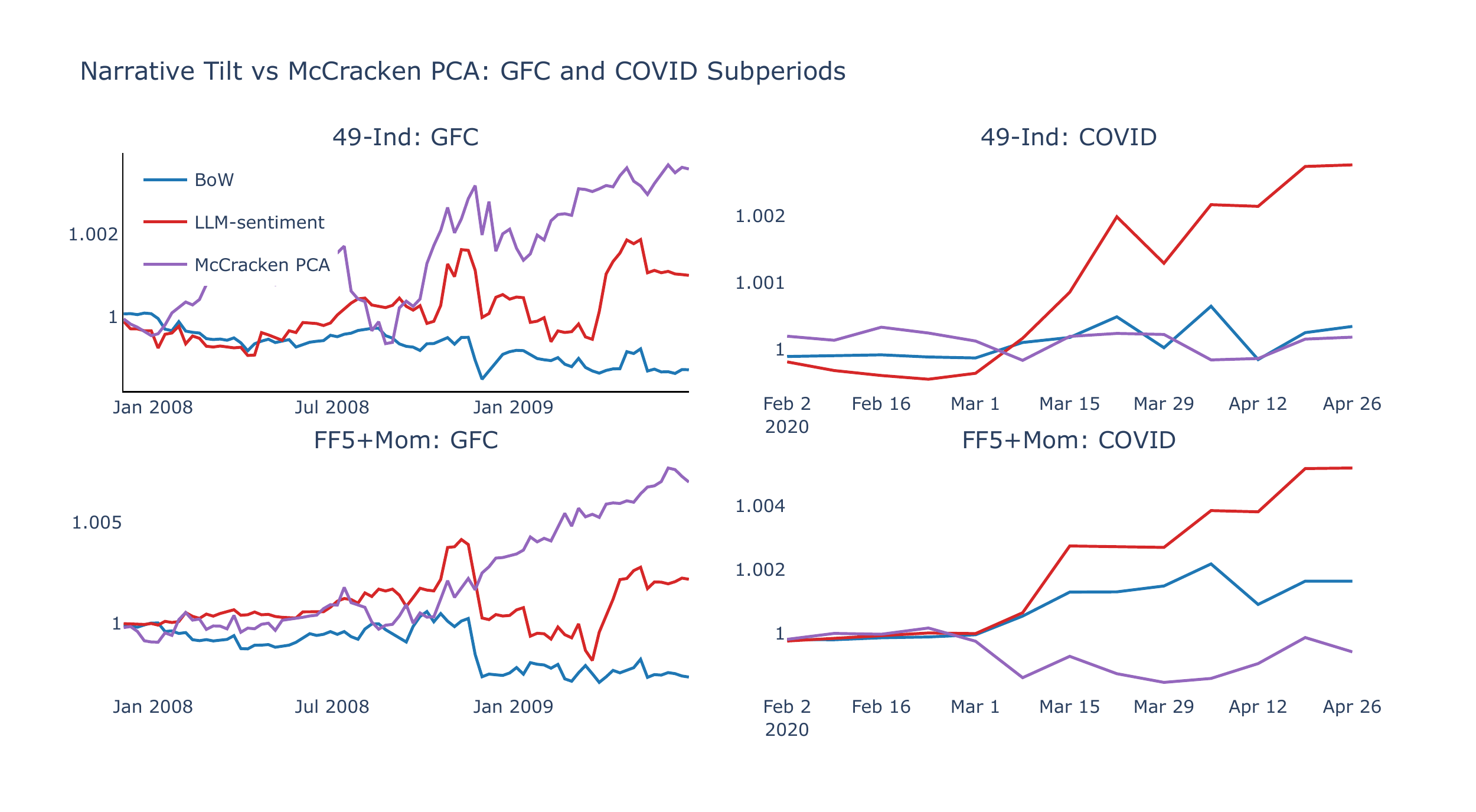
McCracken PCA vs narratives: GFC and COVID
Table A4 compares McCracken PCA CW returns with narrative CW returns during the two major crises.
| Universe | Strategy | Ann. Ret (COVID) | Ann. Ret (GFC) | Sharpe (COVID) | Sharpe (GFC) |
|---|---|---|---|---|---|
| 49-Ind | BoW | 0.001 | −0.001 | 0.53 | −0.74 |
| LLM-sentiment | 0.011 | 0.001 | 3.01 | 0.29 | |
| McCracken PCA | 0.001 | 0.002 | 0.48 | 0.82 | |
| FF5+Mom | BoW | 0.007 | −0.002 | 1.72 | −0.64 |
| LLM-sentiment | 0.021 | 0.001 | 4.09 | 0.37 | |
| McCracken PCA | −0.002 | 0.004 | −0.58 | 1.43 |
Notes. GFC = Dec 2007–Jun 2009; COVID = Feb–Apr 2020. Ann. Ret is annualized from weekly returns. McCracken PCA uses ten FRED-MD principal components (McCracken & Ng, 2016) with expanding betas estimated at monthly frequency from 1970, forward-filled to weekly dates.
During the GFC, the McCracken PCA CW dominates, with Sharpe ratios of 0.82 (49-Ind) and 1.43 (FF5+Mom), while LLM-sentiment is essentially flat (SR \(\approx\) 0) and BoW mildly negative. The slow-moving monthly macro factors—which capture employment, industrial production, and interest rate dynamics—are well-suited to a protracted, fundamentals-driven downturn where bounded narrative sentiment generates negligible \(\Delta\theta\). During COVID, the pattern reverses completely: narrative CW portfolios generate Sharpe ratios of 1.8–5.6, while McCracken is flat (0.48 on 49-Ind) or negative (−0.58 on FF5+Mom). The three-month COVID window is too short for monthly macro data to update meaningfully, whereas daily news narratives adjust within days. Figure A3 illustrates this contrast.
Appendix B. Narrative Momentum Sensitivity
The headline narrative momentum results in Section 4.3 use a composite lookback (12/26/52w), \(J = 5\) narratives per leg, and \(K = 1\) assets per mimicking portfolio. This appendix examines sensitivity to each of these parameters in turn.
Lookback horizon \(M\)
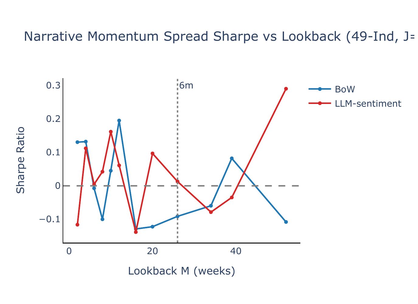
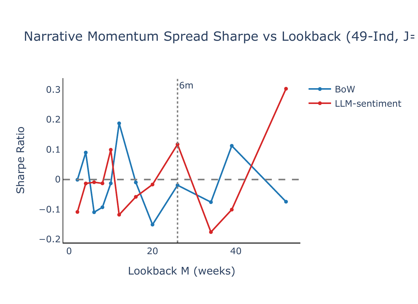
Figure B1 plots the annualised Sharpe ratio of the narrative momentum spread as a function of the lookback horizon \(M\), with \(J = 5\) and \(K = 1\). BoW narrative momentum produces Sharpe ratios near zero or negative across nearly all lookback windows and both universes, while LLM-sentiment exhibits positive Sharpe ratios over most of the grid, with a peak at \(M = 26\) weeks (\(\approx\) 6 months) for FF5+Mom (SR = 0.69, \(t = 3.06\)) and competitive performance at \(M = 52\) weeks for 49-Ind (SR = 0.34, \(t = 1.60\)). The six-month lookback—the headline specification in Lee et al. (2024)—delivers SR = 0.41 (\(t = 1.99\)) on 49-Ind.
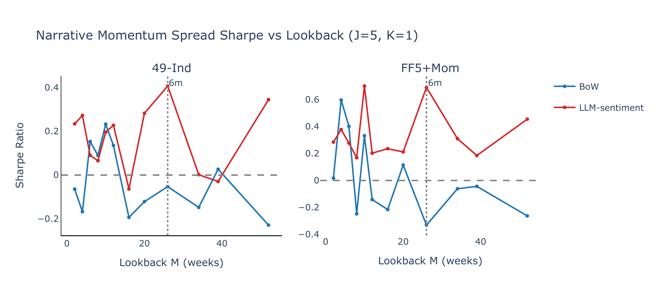
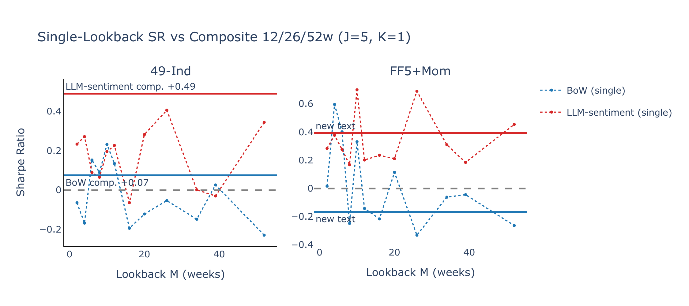
The sensitivity of the LLM-sentiment Sharpe ratio to the choice of lookback—especially on 49-Ind, where it ranges from −0.06 to +0.41—motivates the composite approach described in Section 3.4. Figure B2 compares the single-lookback Sharpe ratios (dotted lines) with the composite signal (horizontal solid lines). For LLM-sentiment, the composite delivers SR = +0.49 (\(t = 2.37\)) on 49-Ind—above the best single lookback—and SR = +0.39 (\(t = 1.70\)) on FF5+Mom. BoW momentum remains flat or negative under the composite, confirming that the BoW–LLM contrast is robust to lookback aggregation.
Narratives per leg \(J\)
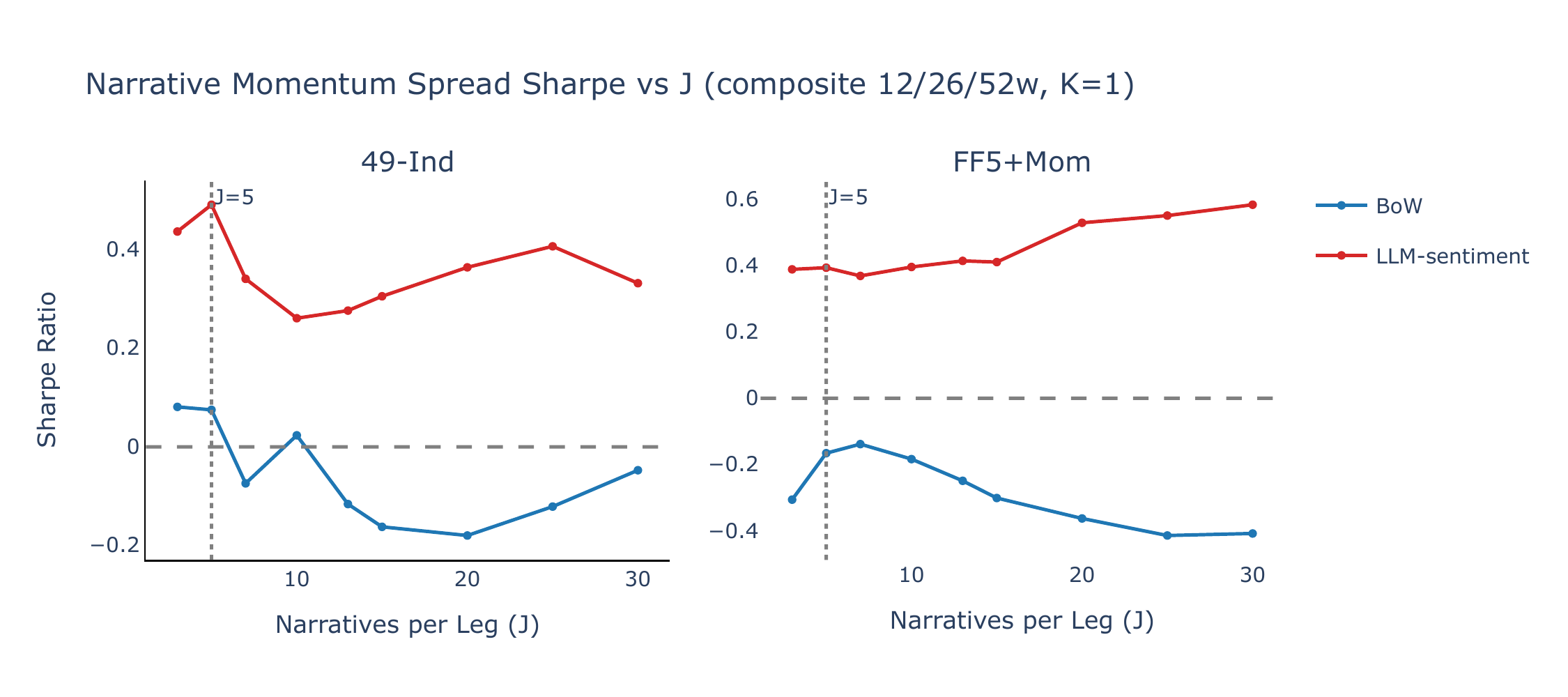
Figure B3 varies the number of narratives per leg (\(J\)) from 3 to 30 while holding \(K = 1\) and using the composite lookback signal (12/26/52w). LLM-sentiment Sharpe ratios are positive across the entire range of \(J\) on both universes; BoW momentum remains flat or negative throughout. The baseline \(J = 5\) sits near the peak for 49-Ind, while FF5+Mom is largely insensitive to \(J\), reflecting the limited cross-sectional dispersion among its five assets.
Assets per mimicking portfolio \(K\)
Figure B4 varies the number of assets per mimicking portfolio (\(K\)) while holding \(J = 5\) and using the composite lookback. \(K = 1\) is clearly optimal: increasing \(K\) dilutes narrative-specific exposure in the mimicking portfolios, and the LLM-sentiment Sharpe ratio on 49-Ind declines monotonically from its peak at \(K = 1\). FF5+Mom constrains \(K \leq 2\) due to its five-asset universe; even moving from \(K = 1\) to \(K = 2\) reduces the spread Sharpe ratio.
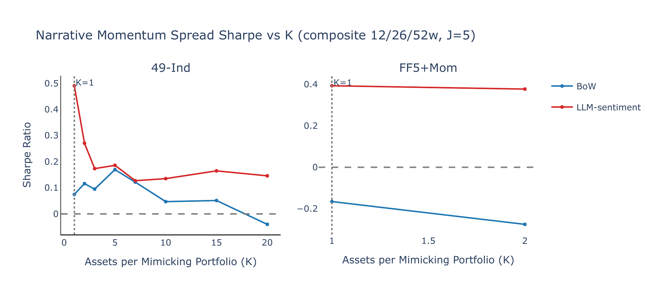
Figures B5–B8 further illustrate the effect of wider mimicking portfolios using single-lookback (\(M = 26\)w) results. Increasing \(K\) from 1 to 10 (\(J = 5\)) eliminates the LLM-sentiment advantage entirely (SR falls from +0.41 to +0.01), while doubling \(J\) to 10 with \(K = 5\) yields only a modest LLM Sharpe of +0.12 (\(t = 0.59\)). These results confirm that \(K = 1\) is the critical design choice: each mimicking portfolio must isolate the single most exposed and least exposed asset to preserve the narrative-specific signal.

Appendix C. Multi-Horizon Composite Signal
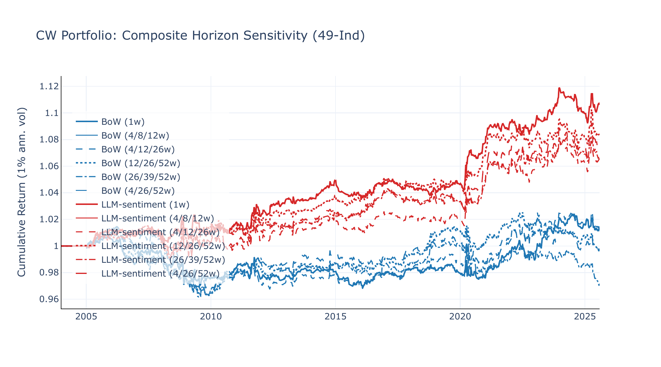
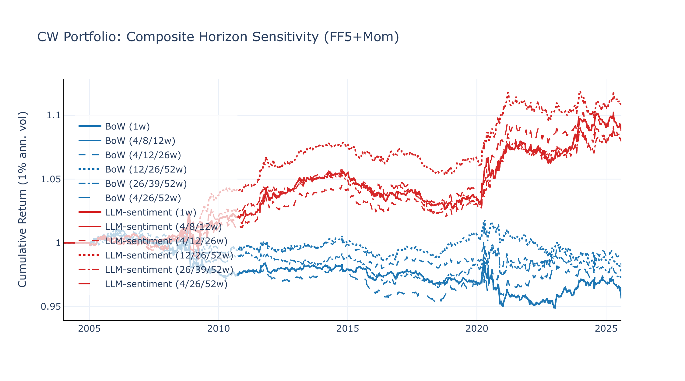
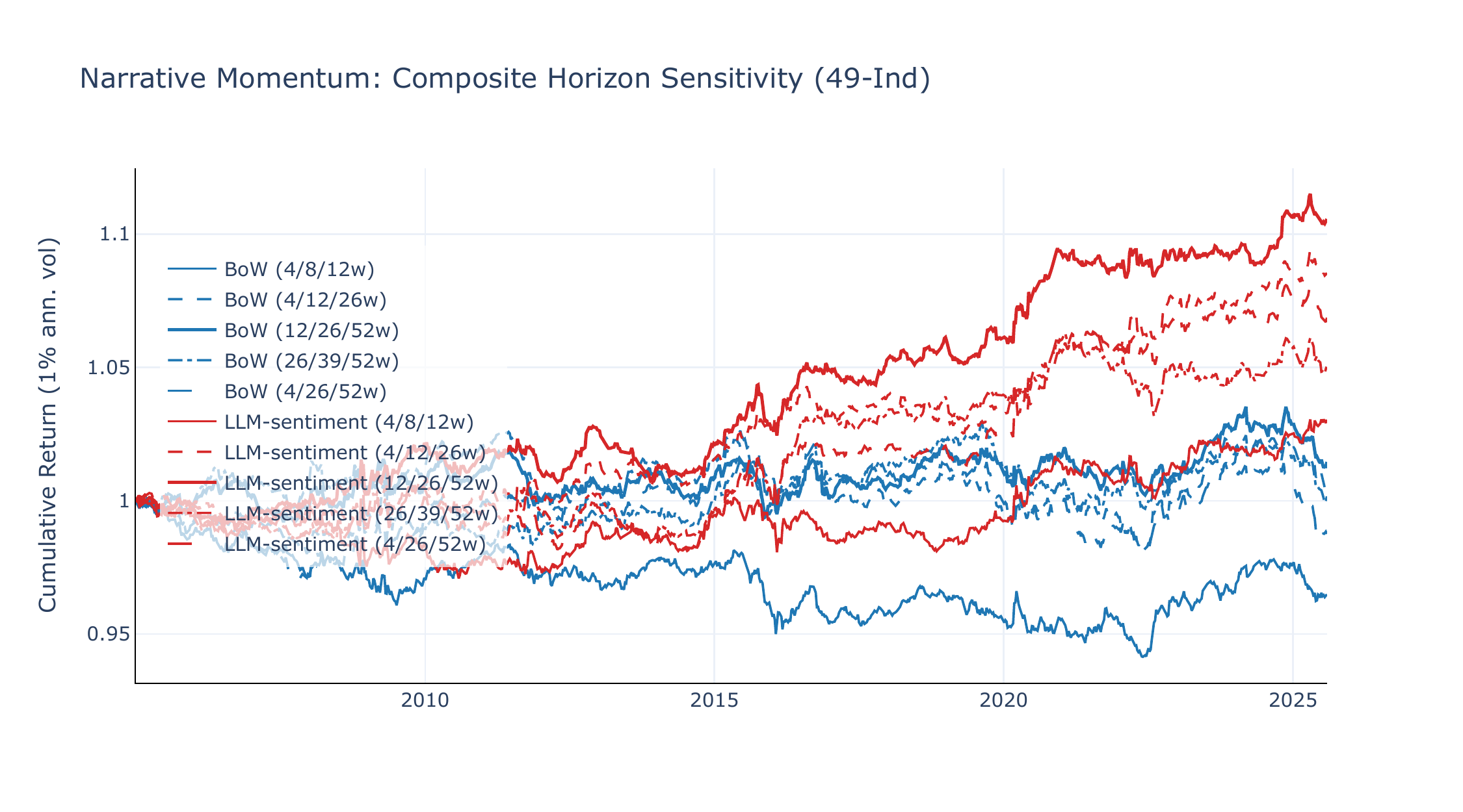
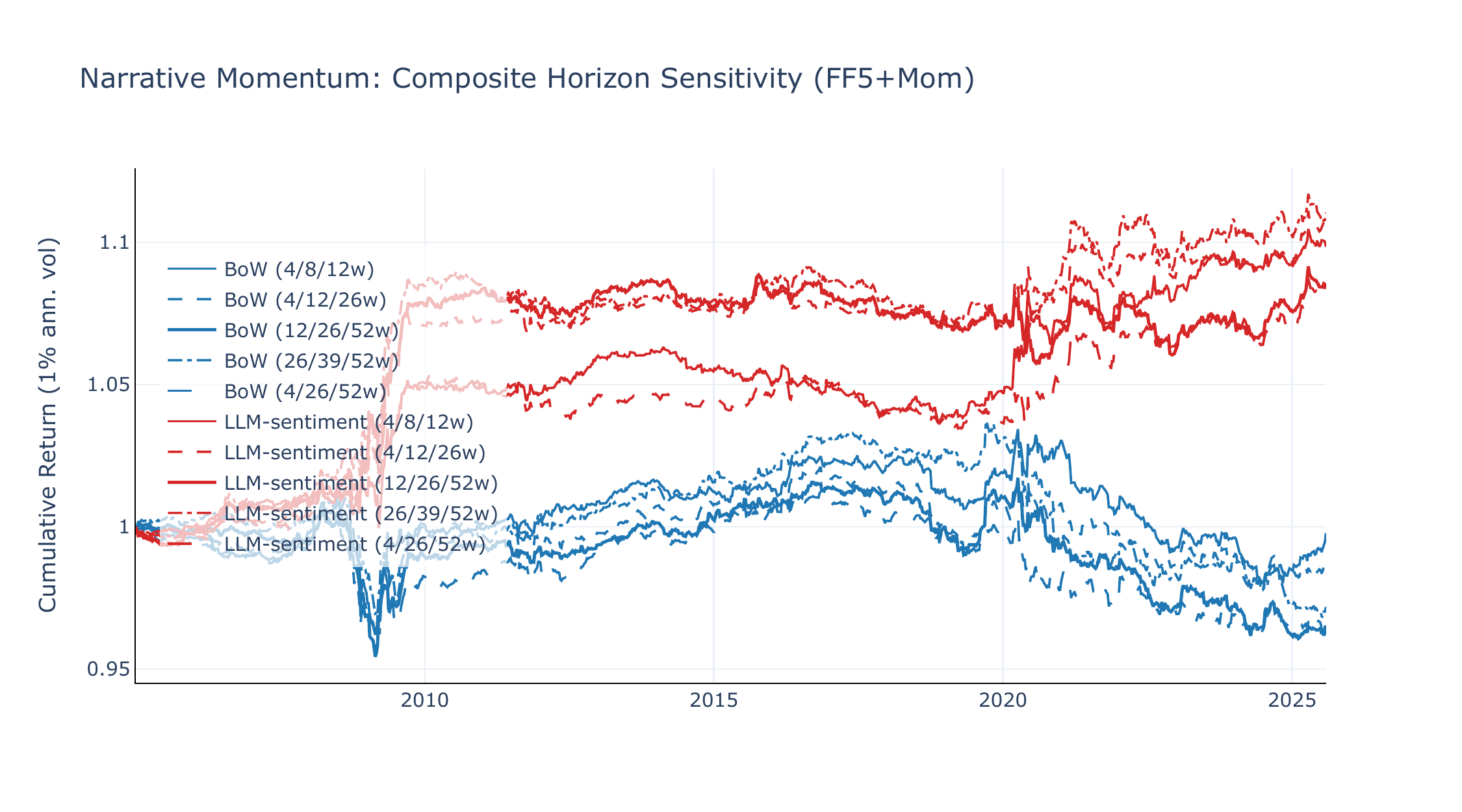
The main text uses a short-horizon composite \(\bar{\Delta}\theta\) with \(\mathcal{H} = \{4, 8, 12\}\) weeks for the CW portfolio and a long composite \(\mathcal{H} = \{12, 26, 52\}\) weeks for narrative momentum. Here we test sensitivity to the composite composition by varying the three lookback horizons while holding the number of lookbacks fixed at three. We consider five specifications: (1) Very short {4, 8, 12}w \(\approx\) 1/2/3 months (CW baseline); (2) Short-tilted {4, 12, 26}w—shifts weight toward recent dynamics; (3) Baseline {12, 26, 52}w \(\approx\) 3/6/12 months (narrative momentum baseline); (4) Long-tilted {26, 39, 52}w—persistent trends only; (5) Wide spread {4, 26, 52}w—maximises horizon diversity.
CW portfolio
Figures C1 and C2 overlay CW equity lines across all five horizon sets. LLM-sentiment is remarkably robust: Sharpe ratios range from +0.29 to +0.48 on 49-Ind and +0.36 to +0.48 on FF5+Mom, with the very short baseline (4/8/12w) performing best on 49-Ind and the long composite (12/26/52w) on FF5+Mom. BoW degrades monotonically with longer horizons, reflecting its reliance on high-frequency count spikes.
Narrative momentum
Figures C3 and C4 compare narrative momentum spreads across the same five horizon sets. The horizon preference is universe-dependent. On 49-Ind, the baseline (12/26/52w) dominates with LLM SR +0.49 (\(t = 2.37\)), while the very short composite (4/8/12w) drops to SR +0.15, indicating that industry-level narrative momentum requires longer lookbacks. The short-tilted (4/12/26w) recovers much of the performance (SR +0.40, \(t = 2.08\)), suggesting that the 26-week horizon carries most of the signal. On FF5+Mom, the pattern reverses: the long-tilted composite (26/39/52w) achieves the highest LLM SR (+0.51, \(t = 2.14\)), but all five specifications deliver SR \(\geq\) +0.39, indicating that factor-level narrative momentum is robust to horizon choice.
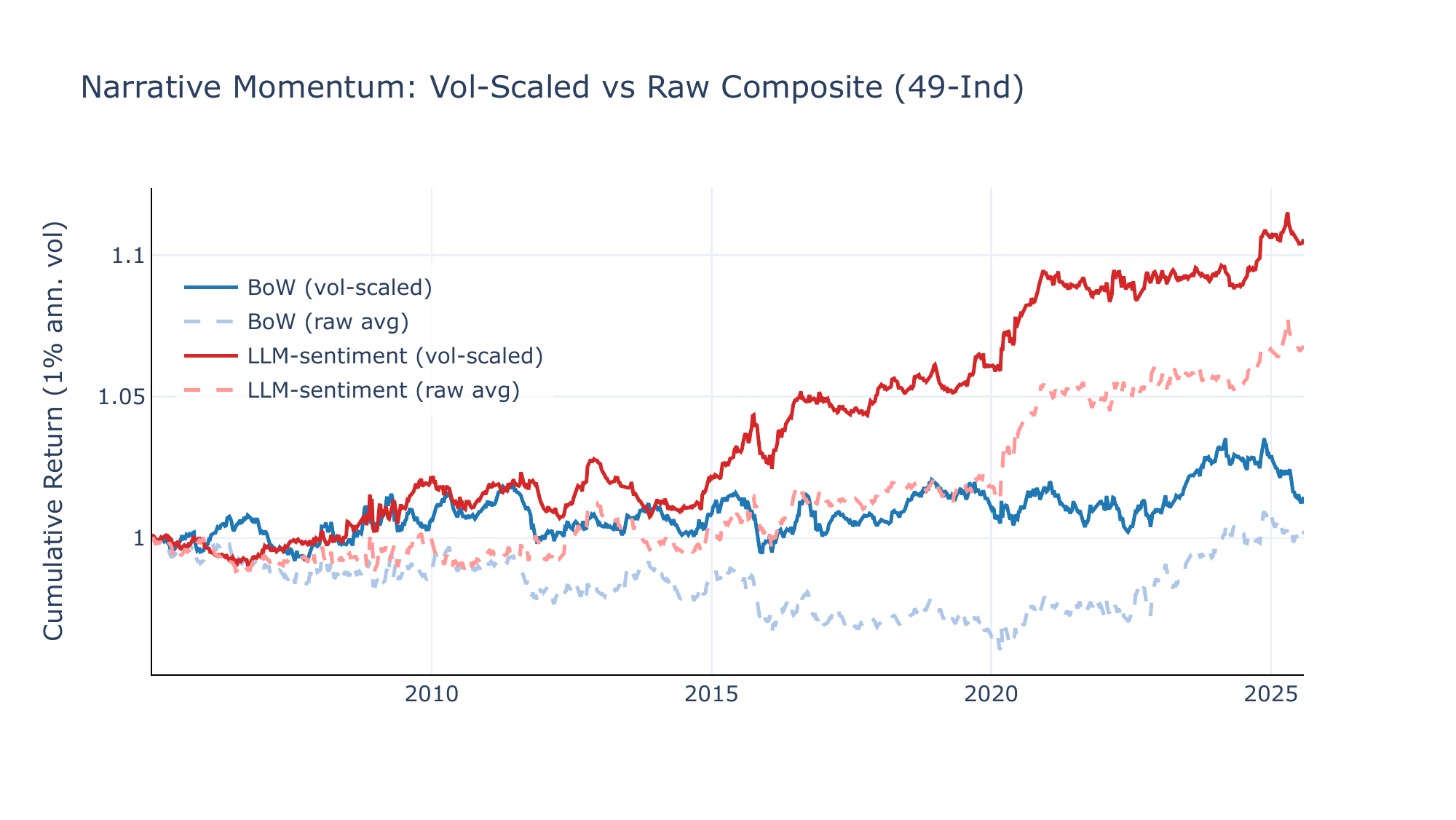
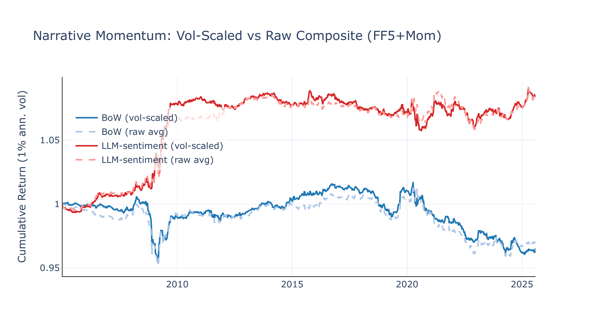
Narrative momentum without vol-scaling
The baseline composite cross-sectionally vol-scales each horizon’s rolling-mean \(\Delta\theta\) before averaging, ensuring all lookbacks contribute equally. Figures C5 and C6 compare the vol-scaled composite with a raw average of rolling means for the baseline horizons (12/26/52w). On 49-Ind, the raw composite is materially weaker (LLM SR +0.32, \(t = 1.60\) vs. +0.49, \(t = 2.37\)), indicating that the vol-scaling step is important for equalising dispersion across horizons when ranking 65 narratives. On FF5+Mom, the two variants are virtually identical (SR +0.39 in both cases), consistent with the smaller cross-section leaving less room for scale differences to matter.
Four findings stand out. First, the LLM-sentiment CW portfolio is insensitive to the composite horizon—SR ranges from +0.29 to +0.48 on 49-Ind and +0.36 to +0.48 on FF5+Mom—while BoW degrades monotonically with smoothing. Second, the two strategies have opposite horizon preferences: the CW portfolio favours short smoothing (preserving high-frequency \(\beta \times \Delta\theta\) variation), while narrative momentum on 49-Ind requires longer lookbacks to identify persistent cross-narrative trends. Third, the short-tilted composite (4/12/26w) offers a reasonable compromise for narrative momentum, recovering \(\sim\)80% of the baseline SR on 49-Ind while slightly improving on FF5+Mom. Fourth, the vol-scaling step matters for narrative momentum on 49-Ind (SR drops from +0.49 to +0.32 without it) but is inconsequential on FF5+Mom, suggesting that normalisation is most valuable when the cross-section is large enough for scale differences across horizons to distort the ranking.
References
- (2016). Measuring economic policy uncertainty. The Quarterly Journal of Economics, 131(4), 1593–1636. https://doi.org/10.1093/qje/qjw024
- (2023). Quantifying narratives and their impact on financial markets. The Journal of Portfolio Management, 49(5), 82–95. https://doi.org/10.3905/jpm.2023.1.472
- (2009). Parametric portfolio policies: Exploiting characteristics in the cross-section of equity returns. The Review of Financial Studies, 22(9), 3411–3447. https://doi.org/10.1093/rfs/hhp003
- (2024). Business news and business cycles. The Journal of Finance, 79(5), 3105–3147. https://doi.org/10.1111/jofi.13377
- (2014). Frog in the pan: Continuous information and momentum. The Review of Financial Studies, 27(7), 2171–2218. https://doi.org/10.1093/rfs/hhu003
- (2024). The macroeconomics of narratives. NBER Working Paper No. 32602. https://doi.org/10.3386/w32602
- (2019). Text as data. Journal of Economic Literature, 57(3), 535–574. https://doi.org/10.1257/jel.20181020
- (2016). … and the cross-section of expected returns. The Review of Financial Studies, 29(1), 5–68. https://doi.org/10.1093/rfs/hhv059
- (2024). Narrative momentum. SSRN Working Paper. https://ssrn.com/abstract=4912496
- (2011). When is a liability not a liability? Textual analysis, dictionaries, and 10-Ks. The Journal of Finance, 66(1), 35–65. https://doi.org/10.1111/j.1540-6261.2010.01625.x
- (2016). FRED-MD: A monthly database for macroeconomic research. Journal of Business & Economic Statistics, 34(4), 574–589. https://doi.org/10.1080/07350015.2015.1086655
- (2017). Narrative economics. American Economic Review, 107(4), 967–1004. https://doi.org/10.1257/aer.107.4.967
- (2007). Giving content to investor sentiment: The role of media in the stock market. The Journal of Finance, 62(3), 1139–1168. https://doi.org/10.1111/j.1540-6261.2007.01232.x